Principle of least action
\(\def \R {\mathbb R} \def \X {\mathcal X} \def \A {\mathcal A} \def \E {\mathcal E} \def \S {\mathcal S} \def \L {\mathcal L} \def \H {\mathcal H}\) Recall that in classical mechanics, the motion of a body under force is governed by Newton’s (second) law of motion:
\[F = ma\]where $F$ is the force acting on the object, $m$ is mass (we can set $m=1$ for convenience), and $a = \ddot X_t$ is acceleration, which is the second derivative of position $X_t \in \X$. Here $\X = \R^d$ is the standard Euclidean space ($d=3$ in physics), but more generally it is a smooth manifold.
In physics, all basic forces are conservative, which means it can be derived as the gradient of a potential energy. For us, this potential energy is given by our optimization objective function:
\[f \colon \X \to \R\]which we assume is convex and smooth. The force is given by the negative gradient:
\[F(x) = -\nabla f(x)\](the negative sign is just by convention, but for our optimization purposes it is important because we want to minimize $f$, so the force points to the steepest descent direction).
Then Newton’s law states that the dynamics of the body is a second-order differential equation:
\[m\ddot X_t + \nabla f(X_t) = 0\]which has a lot of nice properties, for instance, it conserves the total energy (or Hamiltonian):
\[\E_t = \frac{m}{2}\|\dot X_t\|^2 + f(X_t)\]which is the sum of the kinetic and potential energy.
Principle of least action
Newton’s law is a local view of the world: If we know some initial information (e.g., initial position $X_0$ and velocity $\dot X_0$), then we can solve Newton’s equation above to generate the trajectory $X_t$ at any future time $t \ge 0$. So we travel on a unique path as time inexorably flows forward.
It turns out there is also an equivalent global view, in which we are choosing over all possible paths. Specifically, we have to fix initial and final conditions in spacetime:
\[(x_0, t_0), (x_1, t_1) \in \S \cong \X \times \R\]and we consider all possible paths $X \colon [t_0, t_1] \to \X$ interpolating them, so that $X_{t_0} = x_0$ and $X_{t_1} = x_1$. To each such path $X \in \mathfrak{X}$ we associate a value called the action $\A(X) \in \R$, and the rule is to find the best path with the least action:
\[\min_{X \in \mathfrak{X}} \A(X)\]Notice, this is a variational problem over paths, where instead of looking for a special point (like the minimizer $x^\ast$ of $f$), we are looking for an entire path $X = (X_t)$ that minimizes the action $\A$. Therefore, the problem of dynamics of a particle in space now becomes the problem of statics over “strings” or paths of the particle in spacetime.
Even though the action $\A \colon \mathfrak{X} \to \R$ is a functional on an infinite-dimensional space of paths, the rule for minimizing it is still the same: We differentiate $\A(X)$ with respect to $X$ and set it to zero. (So in general we can only make the action stationary, so this is really the “principle of stationary action”, but “principle of least action” sounds more dramatic.)
Euler-Lagrange equation
In general, the action $\A(X)$ is not an arbitrary functional of the path $X \colon [t_0, t_1] \to \X$. Rather, it has the nice property of being the time integral of a quantity called the Lagrangian
\[\L \colon \X \times \R^d \to \R\]along the path $X$, that is, we assume the action has the following form:
\[\A(X) = \int_{t_0}^{t_1} \L(X_t, \dot X_t) \: dt\](Here the domain of the Lagrangian is really the tangent bundle of $\X$. And more generally, in field theory, the action is the integral of a Lagrangian density over spacetime; here we are in the “deterministic” case where the density is concentrated at a single point $X_t$ in space.)
The form above is nice because it says that the action $\A$ has the “disintegration over time” property, and in some sense the Lagrangian $\L$ is its time derivative. This gives an “additivity” or nesting optimality property, whereby the subpath of a least action path must also be a least action path for the intermediate time (this is also the “optimal substructure” property in dynamic programming).
In particular, the first-order optimality condition for the least action path is now given by a differential equation called the Euler-Lagrange equation:
\[\frac{d}{dt} \left( \frac{\partial \L}{\partial \dot x} (X_t, \dot X_t) \right) = \frac{\partial \L}{\partial x} (X_t, \dot X_t)\]Notice carefully what the equation above means, especially on the left hand side: We first take the partial derivative of the Lagrangian $\L(x, \dot x)$ with respect to velocity $\dot x \in \R^d$, then plug in the time-dependent input $(x, \dot x) = (X_t, \dot X_t)$, and finally differentiate with respect to time. The same on the right hand side, except we take partial derivative with respect to space $x \in \X = \R^d$, and we don’t differentiate with respect to time. (So one way of remembering this is that we are differentiating with respect to time an even number of times on each side.)
Specifically, we can calculate the functional derivative of the action $\A(X)$ by making an infinitesimal perturbation $X + \delta \eta$, then using Taylor expansion and integration by parts:
\[\begin{eqnarray*} \A(X + \delta \eta) - \A(X) &= \int_{t_0}^{t_1} \left\langle \frac{\partial \L}{\partial x} (X_t, \dot X_t), \; \delta\eta_t \right\rangle + \left \langle \frac{\partial \L}{\partial \dot x} (X_t, \dot X_t), \; \delta \dot \eta_t \right\rangle dt \\ &= \int_{t_0}^{t_1} \left\langle \frac{\partial \L}{\partial x} (X_t, \dot X_t) - \frac{d}{dt} \frac{\partial \L}{\partial \dot x} (X_t, \dot X_t), \; \delta\eta_t \right\rangle dt \end{eqnarray*}\]where the boundary terms vanish because the test path $\eta$ itself has vanishing endpoints—due to the constraint that $X+\delta \eta$ still interpolate the fixed initial and final conditions $(x_0,t_0)$, $(x_1,t_1)$.
Thus, we see that the functional derivative of $\A(X)$ with respect to the path $X = (X_t)$ is also given by a path that at time $t \in [t_0, t_1]$ takes the value:
\[\frac{\partial \A(X)}{\partial X} \Bigg|_t = \left(\frac{\partial \L}{\partial x} - \frac{d}{dt} \frac{\partial \L}{\partial \dot x}\right) (X_t, \dot X_t)\]Therefore, setting $\partial \A(X) / \partial X = 0$ gives us the Euler-Lagrange equation above, which is a differential equation that has to be satisfied by the optimal path $X$ at each time $t$.
Notice again that this crucially follows from the fact that the action is a time integral of the Lagrangian. If the action were arbitrary, the least action path may have some nontrivial past and future dependence; but because of the disintegration over time property, it turns out the optimal path is characterized by a time-wise differential equation, which is good because it means we can generate its solution over time.
(See also Susskind’s Lecture 3 for an intuitive derivation of the Euler-Lagrange equation by discretizing time.)
So the point is that once we have a Lagrangian $\L(x, \dot x)$, we can calculate the Euler-Lagrange equation above, which is a necessary condition for the curve of least/stationary action defined by integrating $\L$. That is, the Euler-Lagrange equation is the equivalent local view of the global principle of least action.
Newton's law from the ideal Lagrangian
At this point principle of least action may still seem mysterious and complicated, why are we doing it? But it turns out Newton’s law can be equivalently formulated from this perspective. Furthermore (as Susskind explained in Lecture 3), it is a fact of nature that principle of least action turns out to be a solid unifying framework that underlies pretty much everything in physics, from classical mechanics to electromagnetic fields, quantum electrodynamics, standard models of particles, even general relativity.
Concretely, Newton’s law of motion can be recovered from the ideal Lagrangian:
\[\L(x, \dot x) = \frac{m}{2} \|\dot x\|^2 - f(x)\]which is the difference between the kinetic and potential energy. For this Lagrangian, the partial derivative with respect to velocity is momentum:
\[\frac{\partial \L}{\partial \dot x} = m \dot x = p\](indeed this is the proper general definition of momentum), so its time derivative is $\dot p = ma$. Further, the partial derivative with respect to position is force:
\[\frac{\partial \L}{\partial x} = -\nabla f(x) = F\]Thus, the Euler-Lagrange equation $\frac{d}{dt} \frac{\partial \L}{\partial \dot x} = \frac{\partial \L}{\partial x}$ becomes $F = ma$, which is indeed Newton’s law.
(Now we can also ask, why the Lagrangian above? One answer is that it just works to recover Newton’s law. But as Susskind said, it ultimately comes from deep aspects of quantum mechanics—which I don’t understand but sounds cool. And later in his relativity course, Susskind also explained how the kinetic energy in the Lagrangian comes from an expansion of the spacetime metric when the speed of light $c \to \infty$, and this is also where Einstein’s equation $E = mc^2$ comes from. Thus, Newtonian mechanics is an approximation to the Einsteinian theory in the regime of slowly-moving objects.)
Principle of least action has advantages over the Newtonian formulation because it is more intrinsic. Indeed, the statement whether a path minimizes the action is independent of the coordinate system we use to parameterize the problem. So for example, while the equation of motion from Newton’s law may change when we do a coordinate transformation with some fictitious forces arising (e.g., Coriolis and centrifugal forces in polar coordinate), the form is always the same from the Lagrangian perspective, given by the Euler-Lagrange equation, so we can systematically transform the Lagrangian to the new coordinate, then calculate the same Euler-Lagrange equation (see Susskind’s Lecture 3 at 1:03:00).
Furthermore, this Lagrangian approach has a lot of nice mathematical structure. For example, there is the very deep and beautiful Noether’s theorem, which states that there is an equivalence between symmetry and conservation laws in Lagrangian systems. This is manifested, for example, as the conservation of energy, which follows from the fact that the ideal Lagrangian above is time-independent (so it is invariant under the symmetry of time translation).
More directly, we can also see from the Euler-Lagrange equation that if there is a “cyclic” coordinate $x_i$ that does not appear in the Lagrangian $\L$, then the corresponding momentum variable $p_i = \partial \L/\partial \dot x_i$ is conserved since $\dot p_i = \frac{d}{dt} \frac{\partial \L}{\partial \dot x_i} = \frac{\partial \L}{\partial x_i} = 0$.
There is also the equivalent Hamiltonian formulation which works in the phase space of position and momentum. In general, the Hamiltonian $\H(x,p)$ is defined as the Legendre transform (convex conjugate) of the Lagrangian $\L(x,\dot x)$. For the ideal Lagrangian above, the Hamiltonian is equal to the sum of the kinetic and potential energy:
\[\H(x,p) = \frac{1}{2m}\|p\|^2 + f(x) = \frac{m}{2}\|\dot x\|^2 + f(x)\]So in this case the Hamiltonian is equal to the mechanical energy, and it is conserved along the trajectory of the motion.
So now we know the amazing fact that in classical mechanics, objects do not move arbitrarily, but they follow special paths with the least action. At first this may seem baffling. If in the physical world we throw a rock from here to there, how can the rock know to choose the best possible path to do that?
But the key point is that principle of least action requires that we specify boundary conditions (we used this in the integration by parts above to make sure the boundary terms vanish). So we still need the same amount of information to determine a solution: In Newton’s law we need initial position and velocity, while in the principle of least action formulation we need initial and final positions in spacetime. In particular, the initial velocity is no longer an input to the problem, but it is now part of the solution: We need to launch the trajectory with the correct velocity to interpolate from $(x_0,t_0)$ to $(x_1,t_1)$.
(In the rock example above, the path of the rock is the least action path only after we condition on the initial and final positions. This act of choosing the final position also determines the initial velocity, which in turn determines the complete trajectory by Newton’s law. So they are indeed equivalent.)
Friction as damped Lagrangian
In the last post we have seen how friction can be modeled as velocity-dependent force. So we are now considering an equation of motion of the form:
\[m \ddot X_t + m \dot \gamma_t \dot X_t + \nabla f(X_t) = 0\]where $\dot \gamma_t \in \R$ is a general time-dependent weight of the friction or damping term. Recall that classical friction (damped harmonic oscillator) uses linear damping $\gamma_t = ct$, so $\dot \gamma_t = c$ is a constant; while accelerated gradient flow (which is our optimization motivation) uses logarithmic damping $\gamma_t = 3 \log t$, so $\dot \gamma_t = 3/t$ is decreasing with time.
At a fundamental level, there still seem to be some disagreements on how to incorporate friction in the Lagrangian framework appropriately (since friction is a lossy macroscopic description of microscopic phenomena, as we noted last time).
Nevertheless, an effective and common approach is to incorporate friction as damped Lagrangian:
\[\L(x, \dot x, t) = e^{\gamma_t} \left( \frac{m}{2} \|\dot x\|^2 - f(x) \right)\]which is obtained by multiplying the ideal Lagrangian by a time-dependent damping function $e^{\gamma_t}$. Notice that the Lagrangian is now time-dependent. However, we can still form the same principle of least action as above, and find that the least action path is still characterized by the same Euler-Lagrange equation:
\[\frac{d}{dt} \left( \frac{\partial \L}{\partial \dot x}(X_t, \dot X_t, t) \right) = \frac{\partial \L}{\partial x}(X_t, \dot X_t, t)\]For the damped Lagrangian above, the momentum variable becomes time-dependent:
\[\frac{\partial \L}{\partial \dot x}(x, \dot x, t) = m e^{\gamma_t} \dot x\]so that its time derivative has a velocity (i.e., damping) term:
\[\frac{d}{dt} \left(\frac{\partial \L}{\partial \dot x}(X_t, \dot X_t, t)\right) = m e^{\gamma_t} \left( \ddot X_t + \dot \gamma_t \dot X_t \right)\]On the other hand, the force variable also becomes time-dependent:
\[\frac{\partial \L}{\partial x}(x, \dot x, t) = - e^{\gamma_t} \nabla f(x)\]so the Euler-Lagrange equation becomes:
\[e^{\gamma_t} \left( m \ddot X_t + m \dot \gamma_t \dot X_t + \nabla f(X_t) \right) = 0\]Canceling the nonzero $e^{\gamma_t}$ factor then recovers the equation of motion with friction above.
Therefore, we can now say that the accelerated gradient flow equation $\ddot X_t + \frac{3}{t} \dot X_t + \nabla f(X_t) = 0$ comes from the logarithmically-damped Lagrangian
\[\L(x, \dot x, t) = t^3 \left(\frac{1}{2} \|\dot x\|^2 - f(x) \right)\](where we have set the mass to be $m=1$ for convenience). Furthermore, the modified equation
\[\ddot X_t + \frac{r}{t} \dot X_t + \nabla f(X_t) = 0\]which still has the same $O(1/t^2)$ convergence rate for any $r \ge 3$, as explored by SBC’14 in their (ultimately unsuccessful) pursuit of a faster rate, can be seen as coming from the Lagrangian
\[\L(x, \dot x, t) = t^r \left(\frac{1}{2} \|\dot x\|^2 - f(x) \right)\]As Susskind explained in his lecture, this Lagrangian formulation provides an extremely neat packaging of the essential features of our problem. In particular, we recall from last time that for our optimization purposes, we want to optimally control the friction to get the fastest solution. A priori, we may only play with the differential equation directly (e.g., by modifying the damping term, as in SBC’14). But from our perspective, a more principled approach is to consider the damped Lagrangian with a general damping function $\gamma_t$, and try to understand why the logarithmic damping $\gamma_t = 3 \log t$ is good to use. As we shall see later, this also helps us understand how the kinetic and potential energy terms interact in a nontrivial way, especially in the non-Euclidean setting.
However, we also note that the time dependence of the Lagrangian is still confusing, and destroys some of the nice properties of the ideal Lagrangian (for example, conservation of energy). Indeed, the mechanical energy $\E_t = \frac{m}{2}|\dot X_t|^2 + f(X_t)$ is now dissipated, which is appropriate for optimization because we want to converge quickly to the stationary point $x^\ast$ of $f$. However, the mechanical energy above is no longer equal to the Hamiltonian.
The Hamiltonian—which is the proper definition of “energy”—also involves the damping function:
\[\H_t = e^{\gamma_t} \left(\frac{m}{2}\|\dot X_t\|^2 + f(X_t) \right)\]and it is no longer a conserved quantity (but it seems to still be decreasing).
Finally, we also note that the method of Lagrange multiplier for constrained optimization can be seen as a particular case of this Lagrangian framework when the Lagrangian only depends on a variable $\lambda$ (the Lagrange multiplier) and not its derivative $\dot \lambda$, so the Euler-Lagrange equation becomes $\partial \L/\partial \lambda = 0$, i.e., $\L$ is always at a stationary point with respect to $\lambda$, which enforces the constraint.
Bonus: Gradient flow as massless (strong friction) limit
It is classically known that we can view the first-order gradient flow dynamics as the “strong friction” limit of damped second-order Newtonian dynamics. As Villani explained in his book (page 646):
“In mechanics, gradient flows often describe the behavior of damped Hamiltonian systems, in an asymptotic regime in which dissipative effects play such an important role, that the effects of forcing and dissipation compensate each other.”
Concretely, the gradient flow equation $\dot X_t + \nabla f(X_t) = 0$ can be seen as the $\lambda \to \infty$ limit of the damped equation $\ddot X_t + \lambda \dot X_t + \lambda \nabla f(X_t) = 0$. This is perhaps more apparent if we define $m = 1/\lambda$ to be the “mass” of the particle, so the equation of motion becomes
\[m \ddot X_t + \dot X_t + \nabla f(X_t) = 0\]and it is clear that we indeed recover gradient flow in the “massless limit” as $m \to 0$.
Furthermore, note that the equation of motion above comes from the damped Lagrangian
\[\L(x, \dot x, t) = e^{t/m} \left(\frac{m}{2}\|\dot x\|^2 - f(x)\right)\]where the damping function $e^{t/m}$ also scales with $m$. But then the momentum $p = \frac{\partial \L}{\partial \dot x} = me^{t/m} \dot x \to \infty$ as $m \to 0$, which means the particle becomes more massive (has more momentum).
Therefore, gradient flow is the limiting case where the infinitely massive particle simply rolls downhill, and immediately stops at the equilibrium $x^\ast$ as soon as the force $-\nabla f$ vanishes, and there is no oscillation because it is damped by the infinitely strong friction. In this view, moving from a first-order gradient algorithm to a second-order Lagrangian (accelerated) algorithm is faster not by preventing oscillation; rather, it is the opposite, by unwinding the curve to a finite momentum so it can travel faster, albeit with some oscillation.
(Note also that the Lagrangian itself also diverges, $\L \to \infty$ as $m \to 0$, so the first-order gradient flow is really not governed by a Lagrangian, but we can still say it is in the closure of Lagrangian systems.)
What next? Designing the physics of optimization
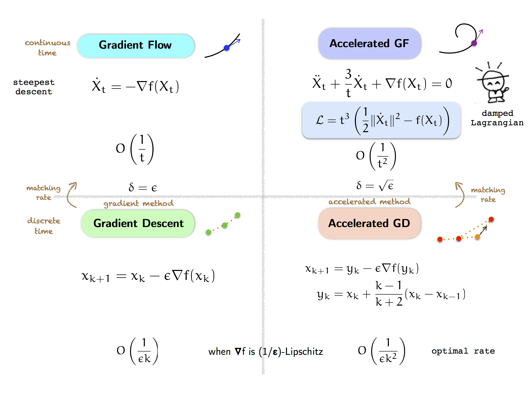
Recall, our optimization motivation is to understand the differences between the first-order gradient flow dynamics (and its corresponding gradient descent algorithm in discrete time) and the second-order accelerated gradient flow dynamics (and its corresponding the accelerated gradient descent algorithm).
Last time, we were confused about where accelerated gradient flow came from. Whereas gradient flow is a simple steepest descent flow, accelerated gradient flow is not intuitive because it is oscillatory, yet has a faster convergence rate ($O(1/t^2)$) than gradient flow ($O(1/t)$) for any convex objective function $f$.
But we now understand that accelerated gradient flow comes from the logarithmically-damped Lagrangian (and our explorer below is happy, because for a brief moment the world makes sense).
So what next? Now we can try to understand further why the damped Lagrangian is good for optimization, and what else we can use. One way to do this is to understand how the Lagrangian generalizes, and in the next post we will start exploring the non-Euclidean case of optimization.
As we shall see, the pattern above—of gradient and accelerated methods in discrete and continuous time—extends to a great generality, both to the non-Euclidean case and to higher-order methods.
This is very interesting, because it tells us of what the “physics” in the world of optimization looks like. The world of optimization is by nature an artificial world, so it doesn’t have a fundamental physical law, and in principle, we can design its physics to be maximally beneficial for our optimization purposes. Yet, from our discussion above and as we shall see further, the physics of accelerated algorithms resembles the physics of the real physical world, via the principle of least action with friction.
Finally, as a closing thought, let us think about optimization in continuous time. If we really want to get a faster convergence rate, what is a simple, obvious idea that should work, but feels like “cheating”? (Hint: We have mentioned this in a previous post.) As we shall see, it turns out that this magical idea actually works! (But interestingly, it only works for accelerated methods, not for gradient algorithms.)
The origin: Part 6