Accelerated gradient flow
\(\def \R {\mathbb R} \def \X {\mathcal X} \def \N {\mathbb N} \def \Z {\mathbb Z} \def \A {\mathcal A} \def \E {\mathcal E}\) Recall that in the world of optimization we have a space $\X = \R^d$ and a convex objective function
\[f \colon \X \to \R\]we wish to minimize.
The basic entity in this world is the gradient descent algorithm:
\[x_{k+1} = x_k - \epsilon \nabla f(x_k)\]which is the simplest algorithm that works in discrete time, in the sense that it minimizes the objective function $f$ at some guaranteed convergence rate under some assumptions on $f$ (such as smoothness).
We have seen there is a corresponding gradient flow dynamics in continuous time:
\[\dot X_t = -\nabla f(X_t)\]which is the simplest dynamics in continuous time that works to minimize $f$ at a matching convergence rate with gradient descent, but under less assumption.
For instance, gradient descent converges at rate $O(1/\epsilon k)$ when $f$ is $(1/\epsilon)$-smooth (that is, $\nabla f$ is $(1/\epsilon)$-Lipschitz, or $|\nabla^2 f(x)| \le 1/\epsilon$), and gradient flow converges at a matching rate of $O(1/t)$ whenever $f$ is convex. The convergence rates match because $t = \delta k$ and $\epsilon = \delta$, where $\delta$ is the discretization time step. Moreover, the smoothness assumption vanishes in continuous time since $1/\epsilon \to \infty$ as $\epsilon \to 0$.
We have also seen the acceleration phenomenon via the accelerated gradient descent algorithm:
\[\begin{array}\; x_{k+1} &= \; y_k - \epsilon \nabla f(y_k) \\ y_k &= \; x_k + \dfrac{k-1}{k+2}(x_k - x_{k-1}) \end{array}\]which achieves a faster—and optimal—convergence rate of $O(1/\epsilon k^2)$ under the same assumption as gradient descent, namely that $f$ be $(1/\epsilon)$-smooth. However, whereas gradient descent is a simple descent method, accelerated gradient descent is oscillatory and less intuitive. Nevertheless, it is interesting that we can achieve a faster convergence rate (in discrete time) not by strengthening the problem assumption, but rather by modifying the base algorithm in a subtle way.
So we have two distinct phenomena that intersect at gradient descent. Then it is natural to wonder whether we can “complete the square”, that is, investigate the phenomenon of acceleration from a continuous-time perspective.
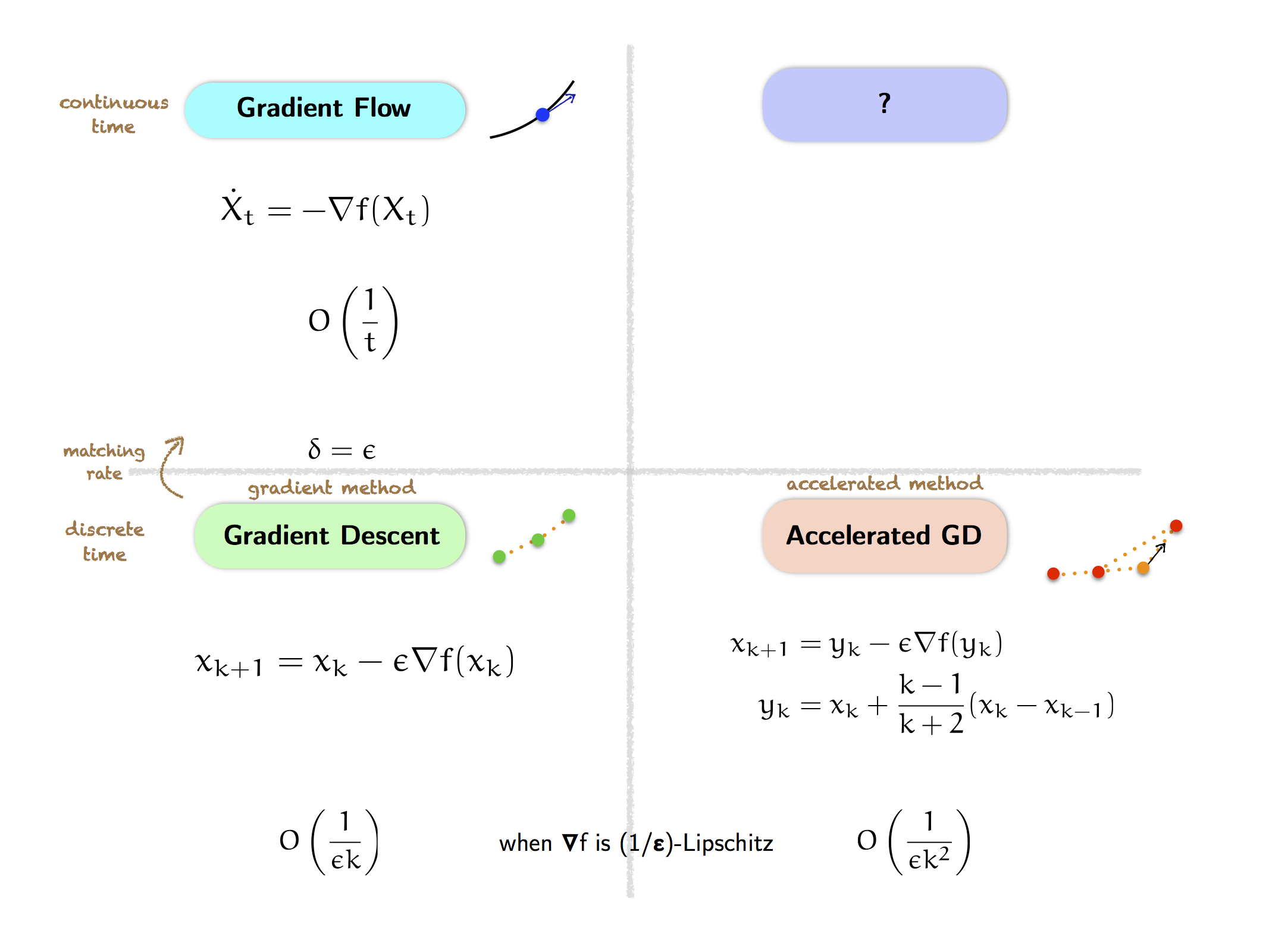
In particular, what is the continuous-time dynamics corresponding to accelerated gradient descent? Is there such a thing as “accelerated gradient flow”, which reflects the acceleration phenomenon in continuous time? Moreover, what convergence rate should we expect accelerated gradient flow to have? If we take the hypothesis of matching structure in continuous time seriously, then given the $O(1/\epsilon k^2)$ convergence rate of accelerated gradient descent, we expect a matching $O(1/t^2)$ convergence rate from accelerated gradient flow (which will imply the scaling $\delta = \sqrt{\epsilon}$ since $t = \delta k$); this turns out to be correct.
Accelerated gradient flow
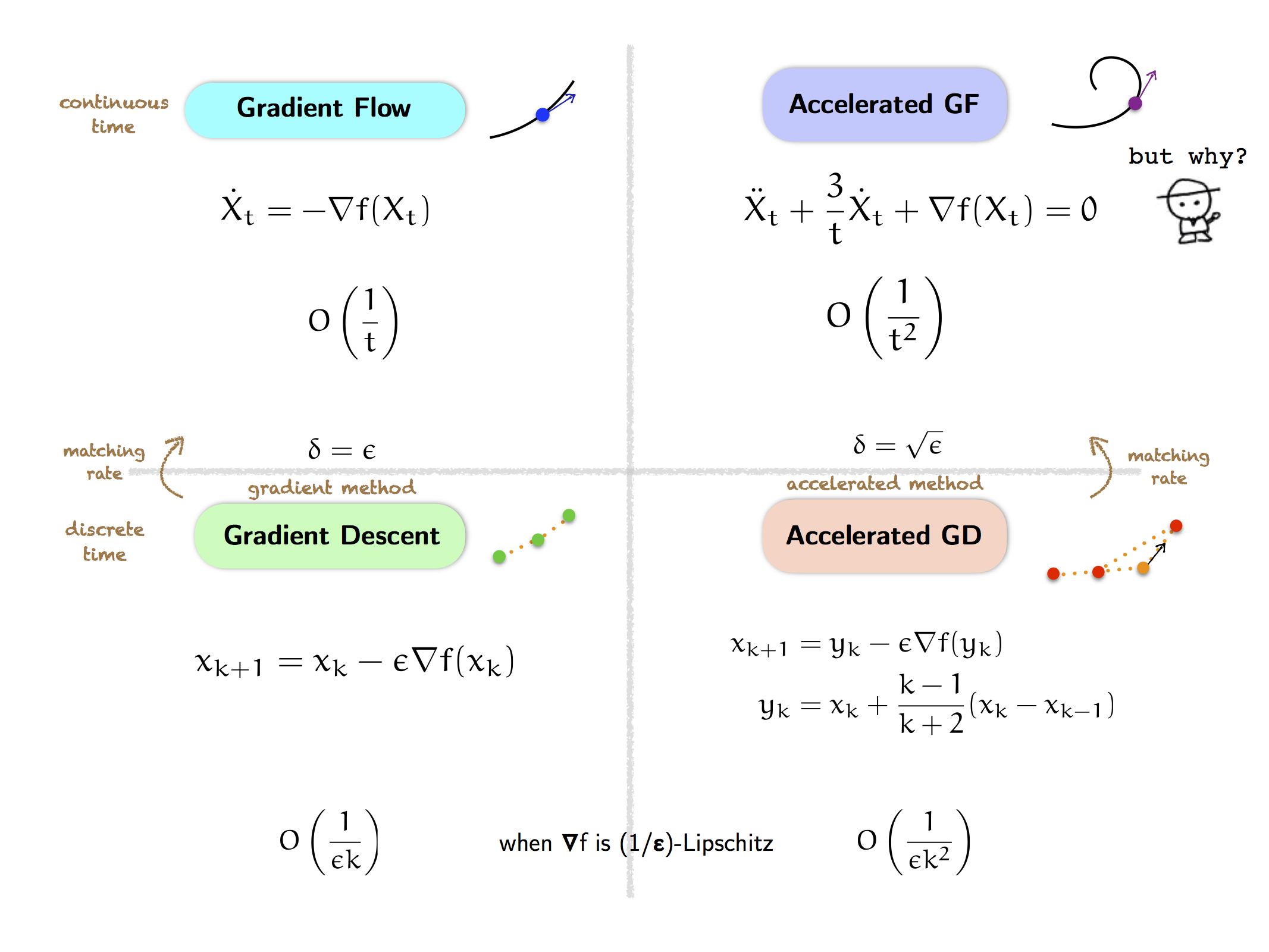
So what is the continuous-time limit of accelerated gradient descent? This is precisely the question studied by Su, Boyd, and Candes (SBC) in their excellent paper that I fortuitously saw at NIPS 2014 and which serves as the main inspiration for our work.
The main result in SBC ‘14 is the following (a priori baffling) fact that the continuous-time limit ($\epsilon \to 0$) of accelerated gradient descent, which is a first-order algorithm, is a second-order differential equation:
\[\ddot X_t + \frac{3}{t} \dot X_t + \nabla f(X_t) = 0\]which, for lack of a better name, we call the accelerated gradient flow. But a posteriori, this fact is not so baffling, and indeed it becomes sort of obvious in hindsight (which is why this result is brilliant). Indeed, accelerated gradient descent is a first-order algorithm in space since it uses the gradient $\nabla f$; on the other hand, accelerated gradient flow is a second-order dynamics in time since it involves the acceleration $\ddot X_t$, but still first-order in space since it only requires the gradient $\nabla f$. Furthermore, the presence of the “momentum” term $x_k - x_{k-1}$ in accelerated gradient descent indicates that we are tracking the changes in the velocity $\dot X_t$, which means we care about its derivative, the acceleration $\ddot X_t$.
Nevertheless, it is still shocking that accelerated gradient flow is a second-order dynamics (rather than first-order like gradient flow, perhaps suitably modified). Why? What is the principle for this dynamics? And why is there the coefficient $3/t$ in the velocity term?
Note that being a first-order dynamics, such as gradient flow, does not mean not having acceleration; indeed it does, but the acceleration assumes a special constrained form determined by the velocity. For example, in gradient flow $\dot X_t = -\nabla f(X_t)$ the acceleration is:
\[\ddot X_t = -\nabla^2 f(X_t) \; \dot X_t\]On the other hand, having a second-order dynamics allows us an “additional degree of freedom” to model the acceleration directly as a more general function of position and velocity, albeit at the cost of a greater complexity (e.g., requiring extra initial conditions).
But note also that first-order and second-order dynamics are essentially equivalent since we can always embed a second-order dynamics $(X_t)$ into a system of first-order dynamics $(X_t, \dot X_t)$, although at the cost of doubling the dimension. This means the “complexity” of the dynamics has to be an important factor in our consideration.
(And I think the difference lies much deeper, that gradient flow uses the metric structure on the space, while accelerated gradient flow uses the symplectic structure via the Lagrangian/Hamiltonian formalism; but we’ll go back to this later.)
Derivation and properties
The derivation of accelerated gradient flow in SBC ‘14 proceeds by taking the “continuous-time limit” $\epsilon \to 0$ of accelerated gradient descent under the ansatz
\[x_k \approx X_{\sqrt{\epsilon} k}\]which means continuous time $t$ is related to discrete time $k$ via the scaling
\[t = \delta k = \sqrt{\epsilon} k\]so the time discretization step $\delta$ is related to the step size $\epsilon$ via
\[\delta = \sqrt{\epsilon}\]just as predicted above (so in particular, $\delta \to 0$ as $\epsilon \to 0$). But let’s keep the time step to be $\delta$ for now and see why $\delta = \sqrt{\epsilon}$ is the natural scaling.
So we suppose there is a smooth (continuously differentiable) continuous-time curve $X_t \in \X$, $t \in \R$, such that for small $\delta \to 0$ and large $t = \delta k \to \infty$, we can identify
\[x_k = X_{\delta k} = X_t\]Then we can replace the next iterate $x_{k+1}$ by the value of $X_{t+\delta}$ at a small time increment away:
\[x_{k+1} = X_{\delta(k+1)} = X_{t+\delta} = X_t + \delta \dot X_t + \frac{\delta^2}{2} \ddot X_t + o(\delta^2)\]where in the last step we have used a second-order Taylor approximation. Similarly, we also have
\[x_{k-1} = X_{\delta(k-1)} = X_{t-\delta} = X_t - \delta \dot X_t + \frac{\delta^2}{2} \ddot X_t + o(\delta^2)\]where notice that we have expanded $X_{t-\delta}$ around $X_t$, so we get negative velocity $\dot X_t$. Thus, we have
\[x_k - x_{k-1} = \delta \dot X_t - \frac{\delta^2}{2} \ddot X_t + o(\delta^2)\]Moreover, since $t = \delta k$, we also have
\[\frac{k-1}{k+2} = 1-\frac{3}{k+2} = 1-\frac{3\delta}{t + 2\delta} = 1-\frac{3\delta}{t} + o(\delta)\]Therefore, we can write the variable $y_k$ in the accelerated gradient descent algorithm as
\[y_k = x_k + \frac{k-1}{k+2} (x_k - x_{k-1}) = X_t + \delta \dot X_t - \delta^2 \left(\frac{3}{t} \dot X_t + \frac{1}{2} \ddot X_t\right) + o(\delta^2)\]Notice that the relation above means the curves $x_k$ and $y_k$ coincide in continuous time ($X_t = Y_t$), since the difference $x_k - y_k = O(\delta)$ is a lower-order term that vanishes as $\delta \to 0$.
Moreover, we can write the gradient at $y_k$ as the gradient at $x_k = X_t$ plus a negligible error:
\[\nabla f(y_k) = \nabla f(X_t + o(1)) = \nabla f(X_t) + o(1)\](however, note that apparently in discrete time we really need $\nabla f(y_k)$ for accelerated gradient descent to work, and we cannot replace it by $\nabla f(x_k)$).
After substituting the approximations above to the accelerated gradient descent algorithm, we obtain:
\[X_t + \delta \dot X_t + \frac{\delta^2}{2} \ddot X_t + o(\delta^2) = X_t + \delta \dot X_t - \delta^2 \left(\frac{3}{t} \dot X_t + \frac{1}{2} \ddot X_t\right) - \epsilon \nabla f(X_t) + o(\delta^2 + \epsilon)\]Notice that the constant and $O(\delta)$ terms above cancel out, which is why we need to do expand up to second-order.
After simplifying, we get the following relation for the dynamics of $X_t$:
\[\delta^2 \left( \ddot X_t + \frac{3}{t} \dot X_t\right) + \epsilon \nabla f(X_t) + o(\delta^2 + \epsilon) = 0\]Now consider how $\epsilon$ should scale as a function of $\delta \to 0$. If $\delta^2 < \epsilon$, then only the first term takes precedence, so $\ddot X_t + \frac{3}{t} \dot X_t = 0$ (which we can solve explicitly), but it is vacuous because it ignores the gradient $\nabla f$ entirely. On the other hand, if $\delta^2 > \epsilon$, then the second term above takes precedence, so $\nabla f(X_t) = 0$, which means $X_t$ is a static curve $X_t = x^\ast$.
Therefore, the only sensible choice to obtain a meaningful dynamics is to set $\delta^2 = \epsilon$, as predicted above, which yields the following second-order differential equation, the accelerated gradient flow:
\[\ddot X_t + \frac{3}{t} \dot X_t + \nabla f(X_t) = 0\]Note that the $3/t$ coefficient in the velocity term above poses a potential singularity problem at $t = 0$. But as observed in SBC ‘14, taking $k=1$ in the definition of accelerated gradient descent forces the dynamics to start with zero initial velocity, $\dot X_0 = 0$, which alleviates the problem at $t = 0$.
Moreover, as shown in SBC ‘14, it turns out we can still prove the existence and uniqueness of the solution $X_t$ to the accelerated gradient flow dynamics, for all time $t \in [0,\infty)$. Although we cannot directly apply standard results (such as the Cauchy-Lipschitz theorem) from differential equations, we can proceed by truncating the $3/t$ term near $t = 0$ and using a uniform approximation argument. (Furthermore, we believe the potential singularity at $t=0$ is in some sense artificial, since the more correct way to write accelerated gradient flow seems to be $\frac{d}{dt}(X_t + \frac{t}{2} \dot X_t) = -\frac{t}{2} \nabla f(X_t)$, see below.)
In any case, we shall not worry about these issues and always assume there is a unique global solution $X_t$ (perhaps under some mild assumption such as $\nabla f$ is Lipschitz), so we can focus on understanding the asymptotic behavior of the solution as $t \to \infty$, which is ultimately what we are interested in.
Furthermore, the heuristic derivation of accelerated gradient flow above can be made more formal, for instance, by defining for each $\epsilon > 0$ a continuous-time curve $X_t^{(\epsilon)}$ that interpolates the discrete-time sequence $x_k$, and showing that the curve $X_t^{(\epsilon)}$ converges (in some appropriate sense) as $\epsilon \to 0$ to the dynamics $X_t$ satisfying accelerated gradient flow.
Indeed, SBC show the following consistency result (in Theorem 2 in their arXiv paper version 2) between accelerated gradient descent and accelerated gradient flow, that for all finite time $T > 0$:
\[\lim_{\epsilon \to 0} \; \max_{0 \, \le \, k \, \le \, T/\sqrt{\epsilon}} \; \|x_k - X_t\| = 0\]This is illustrated in the figures below (Figures 1b and 1c from SBC). The left figure shows the trajectories of the accelerated gradient descent algorithm with small step size $\epsilon$ (denoted by $s$ in the figure), which agree with the true curve of the accelerated gradient flow. The right figure shows that the function values also agree.
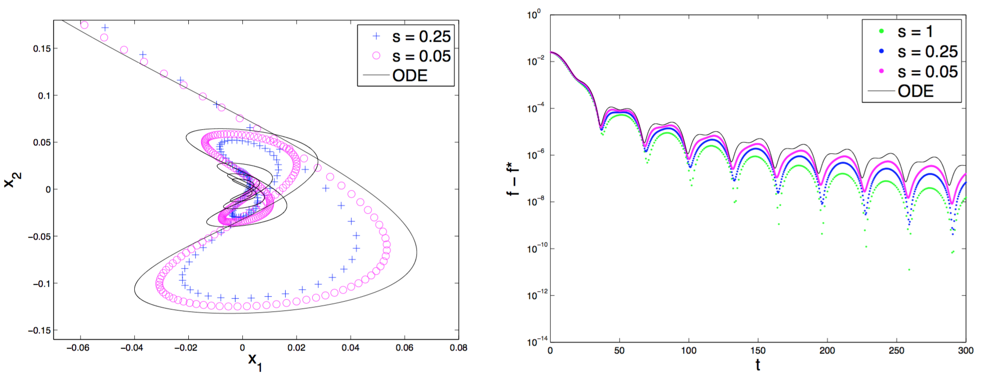
The figures above also clearly show that accelerated gradient flow is an oscillatory dynamics, which means the trajectory of the dynamics on $\X$ oscillates around the minimizer $x^\ast$, and the function value $f(X_t) - f(x^\ast)$ fluctuates up and down. This is in contrast to gradient flow, which is a descent method, so the function value always decreases.
Thus, the contrast between gradient flow and accelerated gradient flow parallels the contrast between gradient descent (which is a descent method) and accelerated gradient descent (which is oscillatory).
Matching convergence rates
A very interesting feature of accelerated gradient flow is that it has a matching convergence rate of $O(1/t^2)$, as predicted above based on the $O(1/\epsilon k^2)$ convergence rate of accelerated gradient descent. Moreover, just like for gradient flow, this convergence rate in continuous time holds whenever $f$ is convex (whereas recall that the convergence rate of accelerated gradient descent requires that $f$ be $(1/\epsilon)$-smooth).
The proof (Theorem 3.2 in SBC ‘14) proceeds by defining the following energy functional:
\[\E_t \equiv \E(X_t, \dot X_t, t) := t^2 (f(X_t) - f(x^*)) + 2\left\|X_t + \frac{t}{2}\dot X_t - x^*\right\|^2\]which serves as a Lyapunov function for the accelerated gradient flow dynamics (i.e., $\dot \E_t = \frac{d}{dt} \E_t \le 0$).
Indeed, by direct calculation and using the key property from the accelerated gradient flow dynamics:
\[\frac{d}{dt} \left(X_t + \frac{t}{2} \dot X_t\right) = -\frac{t}{2} \nabla f(X_t)\]we find that the total time derivative of $\E_t$ is:
\[\dot \E_t = -2t\left(f(x^*) - f(X_t) - \langle \nabla f(X_t), x^* - X_t \rangle \right) \le 0\]where the last inequality follows from the convexity of $f$. This means $\E_t$ is a non-increasing function, so
\[f(X_t) - f(x^*) \,\le\, \frac{\E_t}{t^2} \,\le\, \frac{\E_0}{t^2} \,=\, \frac{2\|X_0-x^*\|^2}{t^2} \,=\, O\left(\frac{1}{t^2}\right)\]The proof above is very simple, and we see that the energy functional is perfectly constructed to complement the accelerated gradient flow dynamics, in particular for the derivative of $X_t + \frac{t}{2} \dot X_t$. However, this poses a question of why $X_t + \frac{t}{2} \dot X_t$ is a good quantity to consider. What is its significance, and why should it converge to $x^*$?
Note that in hindsight, given the dynamics for accelerated gradient flow, it is clear that the energy functional above works to prove the $O(1/t^2)$ convergence rate. But if we were to forget both the accelerated gradient flow dynamics and the energy functional, how would we come up with them in the first place?
In search of a faster rate
One outstanding question from our discussion so far is why the specific form of the accelerated gradient flow dynamics above. In particular, why is it a second-order differential equation, and why do we need the $3/t$ factor in the velocity term?
One possible answer is that it just works, and indeed as we see above, we can prove an $O(1/t^2)$ convergence rate for accelerated gradient flow. But what if we want a faster convergence rate?
In their paper, SBC study a variant of accelerated gradient flow with a more general velocity coefficient:
\[\ddot X_t + \frac{r}{t} \dot X_t + \nabla f(X_t) = 0\]and they show that whenever $r \ge 3$, this new dynamics still has the same $O(1/t^2)$ convergence rate (via a modified energy functional). Thus, there is an apparent “phase transition” at $r = 3$ (see Section 4: “The Magic Constant 3” in their arXiv paper version 2), below which the proof technique breaks down.
It is perhaps comforting that we can perturb the accelerated gradient flow dynamics and still maintain the $O(1/t^2)$ convergence rate. But if we really want to get a faster rate, what should we do? How else should we modify the differential equation?
(As we shall see, the proper way to study a second-order dynamics is not via its differential equation directly, but via its more intrinsic Lagrangian or Hamiltonian representation. In particular, we will see how to achieve a faster convergence rate via the idea of speeding up time, which concretely amounts to weighting the gradient by a time-dependent function, in addition to changing the velocity coefficient.)
When the objective function $f$ is $\mu$-strongly convex, SBC ‘14 show (in Theorem 4.2) that accelerated gradient flow has a faster convergence rate of $O(1/t^3 \sqrt{\mu})$. However, recall (from gradient flow and gradient descent) that for strongly-convex $f$ we typically expect an exponential rate of convergence that depends on the condition number. Furthermore, recall from our discussion in the last post that the form of the accelerated gradient descent algorithm above is only for the smooth case, while the form for the strongly-convex case is slightly different because the coefficients also incorporate $\mu$. Thus, we expect the accelerated gradient flow dynamics above to be valid only for the regular convex case with $O(1/t^2)$ rate, not for the strongly convex case which will require a different form of dynamics.
Indeed, SBC also show that accelerated gradient flow cannot get an exponential rate of convergence, since when $f$ is a quadratic function, we can solve the (modified) accelerated gradient flow equation above to write $X_t$ explicitly in terms of Bessel functions, which yields the rate $f(X_t) - f(x^\ast) = O(1/t^r)$. So somehow the oscillation is preventing us from converging exponentially fast, even when the objective function is very nice like a quadratic. (But again, we will see how to bypass this barrier by speeding up time.)
Another idea that SBC ‘14 propose—building on an earlier approach by O’Donoghue and Candes—is to perform a restart scheme to prevent accelerated gradient flow from oscillating, e.g., by stopping the dynamics and restarting it everytime we detect that the speed is decreasing. This restart scheme turns out to yield a provable exponential convergence rate for accelerated gradient descent (Theorem 5.2). However, the resulting convergence rate is rather complicated and not so natural, since it requires that $f$ be both strongly-convex and smooth in continuous time (whereas usually we only need smoothness in discrete time).
Furthermore, the restart scheme is an artificial intervention layered on top of accelerated gradient flow, which is already a new and mysterious second-order dynamics. We believe it is important to first fully understand the natural dynamics of accelerated gradient flow (without the additional layer of intelligence), and what underlying principles are responsible for its excellent performance for optimization.
But in any case, we now have the following complete square depicting two interesting phenomena in convex optimization: the acceleration phenomenon in discrete time, and the matching parallel structures in continuous time.
We have seen that accelerated gradient flow is a new class of second-order oscillatory dynamics in continuous time, in contrast to gradient flow which is a first-order descent dynamics. We have also seen that there is still a mystery of why accelerated gradient flow works, and what it is actually doing.
A starting point of our work is the basic observation that accelerated gradient flow is the Euler-Lagrange equation of a damped Lagrangian functional, which we will explain next time what it means. This Lagrangian approach allows us to connect our ideas to the principle of least action from physics, and it also gives us a solid foundation with a rich mathematical structure on which to build our theory (in particular, we can draw from the rich literature of calculus of variations and mathematical physics).
The origin: Part 4