Aristotle vs. Newton
\(\def \R {\mathbb R} \def \X {\mathcal X} \def \N {\mathbb N} \def \Z {\mathbb Z} \def \A {\mathcal A} \def \E {\mathcal E}\) Recall that in the world of optimization we have a space $\X = \R^d$ and a convex objective function
\[f \colon \X \to \R\]we wish to minimize. We have seen there are (at least) two kinds of dynamics to solve the optimization problem in continuous time. There is the first-order gradient flow dynamics:
\[\dot X_t = -\nabla f(X_t)\]and there is also the second-order accelerated gradient flow dynamics:
\[\ddot X_t + \frac{3}{t} \dot X_t + \nabla f(X_t) = 0\]These dynamics are interesting to contrast. Whereas gradient flow has a clear and simple interpretation as a greedy steepest descent flow, accelerated gradient flow is not so intuitive because it is oscillatory. Yet, accelerated gradient flow achieves a faster convergence rate of $O(1/t^2)$ whenever $f$ is convex, compared to the $O(1/t)$ rate of gradient flow.
The contrast between gradient flow and accelerated gradient flow is conceptually reminiscent of the difference between Aristotelian and Newtonian physics. As we shall see, adopting this physical perspective yields powerful insights into the behavior of the dynamics in the world of optimization, just as how physics helps us understand (and master) the physical world around us.
In particular, this physical perspective grants us access to the principle of least action, which is an equivalent reformulation of Newtonian (and practically all of) physics from an intrinsic spacetime view, and which will turn out to play a prominent role in our study of accelerated methods in optimization.
As a personal note, let me say that while this post is physics-based, I myself don’t actually have much background in physics. In fact, I have only recently learned about principle of least action via watching Leonard Susskind’s very inspiring lectures in The Theoretical Minimum series, and have since been fascinated by it. (I think had I been aware of it earlier, I would have studied physics in college. But hey, better late than never! :)
In particular, the following is heavily based on Lectures 2 and 3 of the Classical Mechanics course.
Aristotle's law of motion
Aristotle (384-322 BC) developed one of the earliest theories of physics, which unfortunately turned out to be incorrect, but still instructive to understand. As Susskind explained (in Lecture 2):
“The reason Aristotle got it wrong is because he lived in a world dominated by friction. If we apply forces to objects and stop the force, then the object also stops. In a world dominated by friction, an object only moves while there’s a force applied to it. So Aristotle believed that the connection between forces and motions was that the velocity of an object is proportional to a force you put on it.”
Concretely, Aristotle’s hypothesis is that the force $F = F(X_t)$ is related to the velocity $v = \dot X_t$ via:
\[\vec{F} = m \vec{v}\]where $m$ is the mass of the object, which is a constant (we can set $m=1$ for convenience).
However, this is wrong because it doesn’t agree with our everyday experience. As Susskind put it:
“It’s quite clear that Aristotle had never gone ice skating. Had he gone ice skating, he would have realized that it takes force to change motion, or to stop an object.”
Specifically, the problem is that when there is no force ($F=0$), Aristotle’s equation predicts that the velocity is also zero, so the object is static (does not move). Thus, in Aristotle’s view, all objects have a natural resting place where the force vanishes. However, as we experience in ice skating, once we move on ice (with no friction) we can keep moving even without a force, and further, we need to exert a force to stop the motion.
Another problem, which is more philosophical, is that Aristotle’s law fails to be reversible. Here reversibility means that we never lose information, that at a fundamental level we can always retrodict the past as well as predict the future in the laws of physics.
So in what sense is Aristotle’s law irreversible? Susskind illustrated this with the classic example of a spring, in which the force is proportional to the displacement, $F(x) = -kx$ for some $k > 0$. Then Aristotle’s law of motion becomes the first-order differential equation
\[m \dot X_t = -k X_t\]which has an explicit solution
\[X_t = X_0 e^{-\frac{k}{m}t}\]which means regardless of where we start (for any $X_0 \in \X$ at time $t=0$), the trajectory $X_t$ always dereases exponentially fast to the origin (while getting slower, so it only reaches the origin at $t = +\infty$).
So we can predict the future, since everything eventually collapses to the origin. However, we cannot retrodict the past, at least not when we don’t have infinite accuracy. In particular, if we have an object at the origin, can we tell where it came from? If the object is exactly at the origin ($X_t = 0$), then it must have always been there all along. But if we only have a finite precision, then the object may actually be slightly positive or slightly negative (assume $\X = \R$ for now), and these two cases have strikingly diverging histories. (So from this point of view, reversibility is similar to stability in learning theory.)
Notice also that the equation above is identical to the gradient flow equation for the quadratic objective function $f(x) = \frac{k}{2m} |x|^2$. And more generally, Aristotle’s law is identical to gradient flow when the force is the negative gradient of the objective function:
\[F(x) = -\nabla f(x)\](this is called a conservative force, see below).
Finally, it is worth noting that Aristotle’s law may not be actually wrong, but just misunderstood. For example, see this very interesting paper by Carlo Rovelli, in which he shows that (from the abstract):
“Aristotelian physics is a correct and nonintuitive approximation of Newtonian physics in the suitable domain (motion in fluids) in the same technical sense in which Newton’s theory is an approximation of Einstein’s theory.”
However, we shall not pursue this further here, and shall now move on to discuss Newtonian physics. Later, we will see how we can recover gradient flow (and gradient methods in general) as a “strong-friction” or “massless” limit of Newtonian dynamics.
(See also this mind-blowing Nautilus article on how apparently bacteria move following Aristotle’s law!)
Newton's laws of motion
Two millennia after Aristotle’s time, Isaac Newton (1642-1726) developed the theory of universal gravitation and established the foundation of classical mechanics via his famous three laws of motion.
The main conceptual difference is that in Newton’s formulation, the effect of a force $F = F(X_t)$ is not to change velocity directly (as in Aristotle’s), but rather, it is proportional to the acceleration $a = \ddot X_t$:
\[\vec{F} = m \vec{a}\]The above is Newton’s second law of motion, which is the centerpiece of his theory. Newton’s first law is a special case when there is no force ($F=0$), in which case the object moves at a constant velocity. Newton’s third law is equivalent to the conservation of momentum, which follows from a more fundamental principle connecting symmetry and conservation laws, as we shall discuss further later.
In particular, Newton’s laws encompass the principle of inertia: It does not take a force for an object to move; rather, it takes a force to change the state of motion of an object. This is in contrast to Aristotle’s law above, which states that the object has to be static when there is no force, i.e., it has no inertia.
For the spring example above with force proportional to the displacement, $F(x) = -kx$, Newton’s second law becomes the classical harmonic oscillator, which is a second-order differential equation:
\[m\ddot X_t + kX_t = 0\]and which has an explicit sinusoidal solution:
\[X_t = X_0 \cos (\omega t) + \frac{1}{\omega} \dot X_0 \sin (\omega t)\]where $\omega = \sqrt{k/m}$ is the fundamental frequency.
The solution above is periodic and oscillates forever, in contrast to Aristotle’s exponentially-decaying solution. In particular, it is easy to check that the energy is conserved:
\[\E_t \equiv \E(X_t, \dot X_t) := \frac{m}{2} \|\dot X_t\|^2 + \frac{k}{2} \|X_t\|^2\]which means on the $(X_t, \dot X_t)$ space, the sinusoidal solution above moves in a circle (or an ellipse).
Notice also that we now need more initial data to determine a solution. It is not enough to know where we start ($X_0$), but we also need to know how fast we are going ($\dot X_0$). Equivalently, if at time $t$ we are at position $X_t$, then to determine where we will be in the (instantaneous) future $X_{t+\delta}$, we also need to know where we were in the (instantaneous) past $X_{t-\delta}$. Recall, this is in contrast to gradient flow, which has a Markov chain-like property in which the future is determined only by the present, not the past.
All of this also holds more generally. In general, fundamental forces in physics are conservative, which physically means the work done by an object is independent of the path it takes, and concretely means there is a potential function $V(x)$ such that the force is its negative gradient:
\[F(x) = -\nabla V(x)\](In one-dimension, $\X = \R$, we can always define $V$ by integrating $-F$, so all forces are conservative. But in higher-dimension, $\X = \R^d$ with $d > 1$, the condition for a vector field to be the gradient of a function imposes some nontrivial consistency properties—as manifested in the path-independence of work, for instance. Thus, the conservative force hypothesis above is an assumption that will help us mathematically, but it is also a fact in our physical world that fundamental forces are indeed conservative.)
For our optimization purposes, we will take the potential function $V$ to be the objective function $f$:
\[V(x) = f(x)\]Then for a general conservative force
\[F(x) = -\nabla f(x)\]Newton’s second law becomes the second-order differential equation
\[m \ddot X_t + \nabla f(X_t) = 0\]It is easy to verify that the dynamics above conserves the energy:
\[\E_t \equiv \E(X_t, \dot X_t) := \frac{m}{2} \|\dot X_t\|^2 + f(X_t)\]Indeed, by direct calculation, the time derivative of the energy is zero:
\[\dot \E_t = m \langle \ddot X_t, \dot X_t \rangle + \langle \nabla f(X_t), \dot X_t \rangle = 0\]which means $\E_t = \E_0$ stays constant along the trajectory of the dynamics. But this means the dynamics never stops, it perpetually moves, just like the harmonic oscillator example above. Furthermore, since energy is conserved, when the dynamics stops, $\dot X_t = 0$, the potential function $f(X_t)$ has to be at its maximum (along the trajectory). But note that this is the opposite of what we want in optimization, which is to minimize $f$.
And as noted above, since the equation of motion above is a second-order differential equation, we need two pieces of initial data ($X_0$ and $\dot X_0$) to determine the solution. Then it seems like Newton’s law is not completely predictive, since we always need to remember the past to determine the future.
But the “right” way to think about this is to lift the dynamics into a system of first-order equations in a higher-dimensional space. For example, we can consider the configuration space $(X_t, \dot X_t)$ which consists of position and velocity. Or more properly, we can define the momentum variable $p$ by:
\[p_t = m \dot X_t\]and consider the dynamics in the phase space $(X_t, p_t)$. This is the Hamiltonian approach, which has a rich and beautiful mathematical theory using the symplectic structure on the phase space, as we shall discuss further later on.
Finally, we note that in contrast to Aristotle’s law, Newton’s law is indeed reversible. Concretely, this means if we have a solution $X_t$ to Newton’s equation and “run it backward”, i.e., consider the time-reversed curve $Y_t = X_{-t}$, then it is also a solution. This is because when we change the sign of time $t \mapsto -t$, the velocity also flips sign, $\dot Y_t = - \dot X_{-t}$, but the acceleration stays the same, $\ddot Y_t = \ddot X_{-t}$.
Friction (damping)
The Newtonian theory above is nice and beautiful, but nothing in the real physical world moves forever. There is no perpetual motion, since there is friction. This means instead of being conserved, energy is dissipated, so the object gradually loses energy and eventually stops moving.
(When the object comes to rest, it is necessarily at the optimum point where the force vanishes, $\nabla f(x^\ast) = 0$. Thus, interestingly, while friction is “bad” or not ideal in the real world, it is good for our optimization purposes since we want to find the minimizer of $f$ and stay there. So now the problem is, how do we control friction so we get to the optimum as fast as possible?)
So what is friction? As Susskind explained (while pushing an object on a table, at 16:33 in Lecture 2):
Friction is itself a force. When you say the velocity of this object is proportional to the force, what’s really going on, of course, is there are at least two forces applied to this object here. One is my finger, and one is the force of friction. The force of friction is ultimately a microscopic force, or the molecular motions, and all kinds of things which are much too complicated to deal with. So we just call it friction. So it’s really a balance of force. It’s not that the force is necessary to make velocity; it’s just that one force is necessary to overcome the other force.
That is, friction is really a macroscopic description of a system with microscopic degrees of freedom that we are ignoring because they are too complicated or below our precision level. In principle, if we have infinite intelligence and accuracy, then we can take into account all the fundamental interactions and obtain a conservative macroscopic description. But with our limitations, it is often easier to obtain an “effective theory” of the system by brushing out the smaller degrees of freedom. (Effectively, we are considering an open system, since there is the “environment” where the energy is being dissipated to.)
Concretely, friction is typically modeled as a velocity-dependent force:
\[F(x, \dot x) = -c\dot x\]for some constant $c$. In particular, notice that the force is not only a function of position anymore, so we cannot describe it as a vector field on space $\X$ as before.
For example, the spring example above becomes the damped harmonic oscillator equation:
\[m \ddot X_t + c \dot X_t + k X_t = 0\]This equation can be solved explicitly, and the behavior of its solution depends on the “damping ratio” $\zeta = \frac{c}{2\sqrt{mk}}$, as illustrated below (figure from Wikipedia):
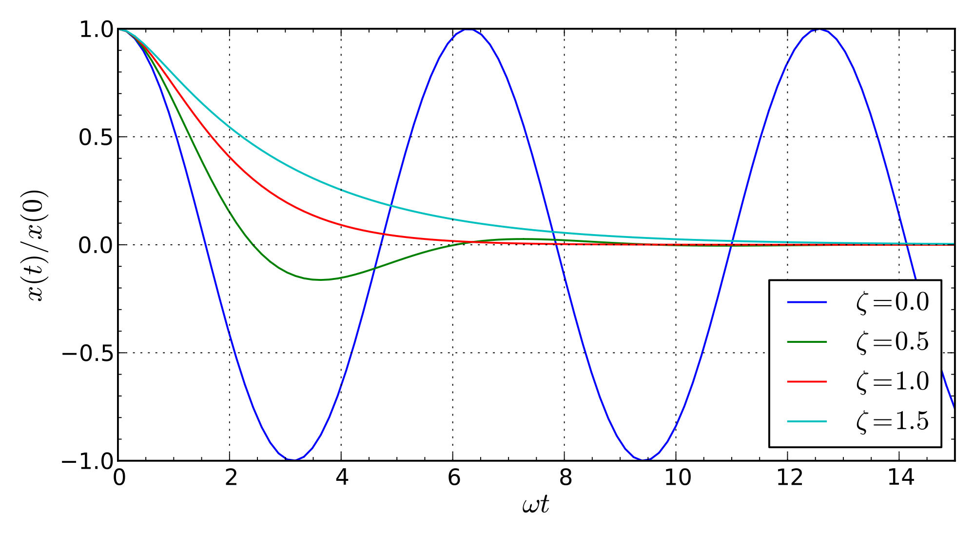
Notice that $c = 0$ (no friction) recovers the sinusoidal solution. For $c > 0$, we see that the solution decays exponentially fast to the origin $0$, which is the minimizer of the objective function $f(x) = \frac{k}{2} |x|^2$.
For a more general objective function $f$, the equation of motion with friction becomes
\[m \ddot X_t + c \dot X_t + \nabla f(X_t) = 0\]It should still be true that the solution converges to the optimum point $x^\ast$ of $f$. For example, we can see that the energy $\E_t = \frac{m}{2} |\dot X_t|^2 + f(X_t)$ (as defined before) is indeed dissipated:
\[\dot \E_t = \langle m\ddot X_t + \nabla f(X_t), \dot X_t \rangle = -c \|\dot X_t\|^2 \le 0\]so $\E_t$ is decreasing along the trajectory of the solution. However, for a general convex function $f$, we cannot prove a guaranteed convergence rate for how fast the convergence $f(X_t) \to f(x^\ast)$ happens.
Back to accelerated gradient flow
Now recall our original motivation of understanding accelerated gradient flow:
\[\ddot X_t + \frac{3}{t} \dot X_t + \nabla f(X_t) = 0\]Notice that the difference between this equation and the classical friction equation above is that here we replace the damping factor from $c$ to a time-dependent function $3/t$.
It is still unclear why we need to do so, since it makes the equation more complicated. Yet, somehow we now have a guaranteed convergence rate under the minimal assumption that $f$ be convex:
\[f(X_t) - f(x^*) \le O\left(\frac{1}{t^2}\right)\]Recall that the proof is via exhibiting an appropriate energy functional that serves as a Lyapunov function for the dynamics. But rather than just the mechanical energy as considered above, the energy functional that we need now involves a scaled version of $f$:
\[\E_t = t^2 (f(X_t) - f(x^*)) + 2\left\|X_t + \frac{t}{2}\dot X_t - x^*\right\|^2\]so that knowing $\E_t$ is decreasing automatically gives us an $O(1/t^2)$ convergence rate. Recall also that the bound above still holds if we further replace the damping coefficient $3/t$ by $r/t$, for any $r \ge 3$.
We hope our discussion here helps us understand accelerated gradient flow a bit more. Although we may still not understand why it works, at least we now have some idea of the connection between accelerated gradient flow and damped Newtonian dynamics. This will allow us to leverage the nice theories that have been developed for Newtonian mechanics (and mathematical physics in general).
In particular, what we will find very useful is the framework of the principle of least action, which reformulates Newtonian mechanics from a global spacetime perspective and captures the intrinsic properties of the dynamics. For example, it is well-known that in Newtonian mechanics there are some “fictitious forces” that arise due to our choice of coordinate system, e.g., Coriolis and centrifugal forces due to Earth’s rotation. These fictitious forces are notoriously difficult to handle directly, but in the least action formulation they arise automatically as the result of a systematic calculation.
The point we wish to make is that rather than working at the level of differential equations (e.g., by modifying the damping coefficient and seeing what happens), we should think at a more fundamental level, using what is called a Lagrangian functional governed by the principle of least action (also equivalent to the Hamiltonian formalism mentioned above). This way, we can reason and work with only the intrinsic properties of the dynamics, which are independent of how we parameterize the problem.
In particular, will see how we can incorporate friction as damped Lagrangian. Then classical friction corresponds to linear damping, while accelerated gradient flow corresponds to logarithmic damping. So somehow logarithmic damping works to give us the logarithmic $O(1/t^2)$ convergence rate. Further, it turns out that by weighting the force term, linear damping also works to give us a linear $O(e^{-ct})$ rate! But more on this next time.
And as a closing thought, let us ponder that from this perspective, what Nesterov did was essentially bringing us from the dark age of Aristotelian physics to the renaissance of Newtonian physics, in the world of optimization.
The origin: Part 5