The world of optimization

$\def \R {\mathbb R} \def \X {\mathcal X} \def \T {\mathbb T}$ In the world of optimization, we have a space $\X$ and an objective function that we wish to minimize:

$$f \colon \X \to \R$$

The space $\X$ is a continuous smooth manifold. For simplicity, unless stated otherwise, we consider

$$\X = \R^d$$

the $d$-dimensional real Euclidean space, for some $d \ge 1$, with the $\ell_2$-norm $|x|^2 = \langle x, x \rangle = \sum_{i=1}^d x_i^2$ .

We assume $f$ is smooth (differentiable as necessary), and there exists a unique global minimizer

$$x^* = \arg\min_{x \in \X} \: f(x)$$

which has the property that the gradient (vector of partial derivatives) vanishes:

$$\nabla f(x^*) = \left( \frac{\partial f}{\partial x_1}(x^*), \dots, \frac{\partial f}{\partial x_d}(x^*)\right) = 0$$

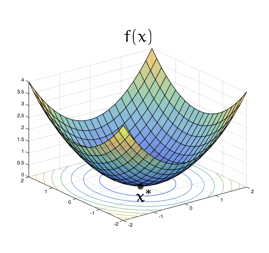
When the objective function $f$ is convex (as illustrated in the picture above for $d=2$), the necessary condition $\nabla f(x^\ast) = 0$ is also sufficient to ensure that $x^\ast$ is the unique global minimizer of $f$.

Thus, convex functions enjoy a nice local-to-global property, in which the local condition of vanishing gradient is equivalent to the global guarantee of being the unique global minimizer:

$$\nabla f(x^*) = 0 ~~\Leftrightarrow~~ x^* = \arg\min_{x \in \X} \: f(x)$$

This property is fundamental in the development of both theory and practice of convex optimization. For instance, the local-to-global property implies that a simple greedy method (such as gradient descent) already provably works to find the minimizer, so it gives us a starting point to develop new algorithms.

However, this nice property is lost when $f$ is nonconvex, since $x^\ast$ may only be a local optimum or saddle point. So nonconvex optimization is a difficult (but important) frontier, and indeed there have been many brave souls who wander off the convex path. But we’ll follow the convex path for now.

The design problem for convex optimization

Given a convex objective function $\;f \colon \X \to \R$, the design problem for convex optimization is the task of designing a fast algorithm to solve the convex optimization problem

$$\min_{x \in \X} \: f(x)$$

Here we measure the speed of an algorithm via the convergence rate $R(k)$ of the function values:

$$f(x_k) - f(x^*) \le O\left(e^{-R(k)}\right) \qquad\text{as}~~k \to \infty$$

so a larger convergence rate means faster convergence. Two major classes of convergence rates are:

• Sublinear (logarithmic) rate: $R(k) = p \log k$ for some $p > 0$, so

  $$f(x_k) - f(x^\ast) \le O\left(\frac{1}{k^p}\right)$$

  This is sometimes also called polynomial convergence rate.

• Linear rate: $R(k) = ck$ for some $c > 0$, so

  $$f(x_k) - f(x^\ast) \le O(e^{-ck})$$

  This is sometimes also called exponential convergence rate.

In general, to have a provable convergence rate we need to impose some assumptions on the problem. Typically there are two classes of assumptions, corresponding to the two convergence rates above:

• Smoothness: Upper bound on curvature, needed for logarithmic convergence rate.

• Strong (uniform) convexity: Lower bound on curvature, needed for linear convergence rate.

We illustrate this with the following basic example, which serves as our foundational building block.

Gradient descent

The simplest algorithm that works for optimization is gradient descent, which is an algorithm that at each iteration takes a step (with a fixed step size $\epsilon > 0$) along the direction of negative gradient:

$$x_{k+1} = x_k - \epsilon \nabla f(x_k)$$

Gradient descent—with its multitude of variants including stochastic, asynchronous, variance-reduced, gradient-free, etc.—is the cornerstone of our world of optimization. Indeed, practically all our algorithms for optimization are derived from the basic greedy principle of following the negative gradient, which is the direction of steepest descent.

In particular, gradient descent is a descent method, which means the function value always decreases:

$$f(x_{k+1}) \le f(x_k)$$

In Nesterov’s excellent book on convex optimization, this property is called a relaxation sequence.

Under additional assumptions, we can further characterize a convergence rate for $f(x_k)$. In particular:

• If $f$ is smooth, which means its gradient $\nabla f$ is Lipschitz:

  $$\|\nabla f(x) - \nabla f(y)\| \le L \|x-y\|$$

  for some $L > 0$, or equivalently, its Hessian $\nabla^2 f$ is bounded above:

  $$\|\nabla^2 f(x)\| := \lambda_{\max}(\nabla^2 f(x)) \le L$$

  then gradient descent with step size $\epsilon = 1/L$ has logarithmic convergence ($R(k) = \log k$):

  $$f(x_k) - f(x^*) \le \frac{2L\|x_0-x^*\|}{k+4} = O\left(\frac{L}{k}\right)$$

  This classic result can be found in, for example, Corollary 2.1.2 of Nesterov ‘04.

  For our purposes, it will be convenient to write the Lipschitz constant $L = 1/\epsilon$ and let the step size $\epsilon > 0$ be the fundamental parameter that governs the algorithm. Thus, we can state the result as:

  Theorem: For all $\epsilon > 0$, if $f$ is $(1/\epsilon)$-smooth, then gradient descent has convergence rate

  $$f(x_k) - f(x^*) \le O\left(\frac{1}{\epsilon k} \right)$$

  This is the basic structure of gradient descent that we will keep in mind. Note in particular the interplay between the assumption ($(1/\epsilon)$-smoothness) and conclusion ($O(1/\epsilon k)$ convergence rate).

  We also remark that the proof essentially hinges on showing the following inequality:

  $$\frac{1}{\Delta_{k+1}} \ge \frac{1}{\Delta_k} + \frac{\epsilon}{2\|x_0-x^*\|^2}$$

  where $\Delta_k := f(x_k) - f(x^\ast)$ is the function value residual; see page 69 of Nesterov ‘04. (But this proof is already not intuitive: what is the significance of the quantity $1/\Delta_k$ and why is it increasing?)

• If $f$ is also strongly convex, which means its Bregman divergence is lower bounded by a quadratic:

  $$D_f(y,x) := f(y) - f(x) - \langle \nabla f(x), y-x \rangle \ge \frac{\sigma}{2}\|x-y\|^2$$

  for some $\sigma > 0$, or equivalently, its Hessian matrix is bounded below:

  $$\lambda_{\min}(\nabla^2 f(x)) \ge \sigma$$

  then gradient descent with step size $\epsilon = 1/L$ has linear convergence ($R(k) = \frac{\kappa}{2} k$):

  $$f(x_k)-f(x^*) \le \frac{\|x_0-x^*\|^2}{\epsilon \; \left(1+\frac{\epsilon \sigma}{2}\right)^k} = O\left(\frac{1}{\epsilon} \exp \left(-\frac{\kappa}{2} k \right)\right)$$

  where

  $$\kappa = \epsilon \sigma = \frac{\sigma}{L}$$

  is the (inverse) condition number which we assume is small, $\kappa \approx 0$. The constant factor can be improved, but more important is the dependence of the convergence rate on the condition number $\kappa$, and the fact that to get linear convergence rate we need both smoothness and strong convexity.

• We note there is also a third class of results for when $f$ is non-smooth and Lipschitz, which means

  $$\|f(x)-f(y)\| \le L \|x-y\|$$

  for some $L > 0$, or equivalently, the gradient $\nabla f$ is bounded,

  $$\|\nabla f(x)\| \le L$$

  in which case gradient descent with a decreasing step size $\epsilon_k \propto 1/\sqrt{k}$ converges at a slower logarithmic rate ($R(k) = \frac{1}{2} \log k$):

  $$f(x_k)-f(x^*) \le O\left(\frac{L}{\sqrt{k}} \right)$$

  which turns out to be the optimal rate for the class of non-smooth functions; see Section 3.2 of Nesterov ‘04. However, we will not discuss the non-smooth case further. For now we focus on exploring the nice structure of the simple case when $f$ is smooth and differentiable.

Footnote: Why optimization?

We live in the era of Big Data, and the promise of Machine Learning is that we can learn structure from data. Indeed, we now have many magical things like face recognition that algorithms can do really well:

(The algorithm misses Angelina and Jared, but it’s still impressive that it recognizes everyone else.)

At an abstract—and simplistic—level, we can formulate machine learning as optimization. This is because when we have a learning task we evaluate the performance of our algorithm via some cost function. Thus, the task of learning can be reduced to the problem of finding the best parameter that optimizes the objective cost function.

In this point of view, the goal of learning is encoded in the design of the objective function. By choosing objective functions with different structure, we can enforce the solution of the optimization problem to have certain regularity properties. For example:

• Ridge regression uses the quadratic loss and $\ell_2$-regularization, which results in a smooth solution.

• Lasso uses $\ell_1$-regularization, which results in a sparse solution.

• SVM (support vector machine) uses the hinge loss, which results in a max-margin solution.

This framework also includes many other classical machine learning algorithms. Furthermore, in all these examples the objective functions are indeed convex, so the theory of convex optimization is essential.

Thus, we are now interested in the problem of convex optimization

$$\min_{x \in \X} \: f(x)$$

in the simple general setting (deterministic, unconstrained, smooth, convex). This may seem too simple, but as we will see, there is a lot of nice structure we can explore and already so much we don’t understand. Having a solid understanding of the simple case will help us build up toward more complex practical problems.

So as a famous man once said, let’s catch the trade winds in our sails. Let us explore. Dream. Discover.

The origin: Part 1