Accelerated gradient descent

$\def \R {\mathbb R} \def \X {\mathcal X} \def \N {\mathbb N} \def \Z {\mathbb Z} \def \A {\mathcal A} \def \E {\mathcal E}$ In the world of optimization, we have a space $\X = \R^d$ and a convex objective function

$$f \colon \X \to \R$$

we wish to minimize. We have seen that gradient descent is a simple greedy algorithm that works to minimize the objective function at some convergence rate (in this post we shall remain in discrete time).

But the world is always stranger than we think.

Indeed, there is a phenomenon of acceleration in convex optimization, in which we can boost the performance of some gradient-based algorithms by subtly modifying their implementation.

In particular, we will discuss accelerated gradient descent, proposed by Yurii Nesterov in 1983, which achieves a faster—and optimal—convergence rate under the same assumption as gradient descent.

Acceleration has received renewed research interests in recent years, leading to many proposed interpretations and further generalizations. Nevertheless, there is still a sense of mystery to what acceleration is doing and why it works; these are the questions that we want to understand better.

Motivation: Can we optimize better?

What is nice about convex optimization is that a simple local greedy algorithm such as gradient descent

$$x_{k+1} = x_k - \epsilon \nabla f(x_k)$$

already works to minimize $f$ (at a guaranteed convergence rate of $O(1/\epsilon k)$ when $f$ is $(1/\epsilon)$-smooth).

But can we do better?

Surely if we devote our creative mind to it, we should be able to design a better, faster algorithm that is doing something more clever than just “going downhill” like gradient descent, right? But how?

Consider for example that gradient descent is a relaxation sequence (descent method), which means the objective function always decreases:

$$f(x_{k+1}) \le f(x_k)$$

This is a natural property to have for optimization, and it is crucial for the analysis of gradient descent.

If our algorithm satisfies the relaxation property, then it is natural to choose the next point $x_{k+1}$ to maximize the decrease in the objective function $f$. But then we essentially end up with gradient descent.

That is, gradient descent is already the “optimal” relaxation method. But recall, our goal is to improve it.

So it seems like we should abandon the relaxation sequence property. This sounds like a radical idea, because if our goal is to minimize $f$, why should we allow $f$ to increase at all? But amazingly, it works.

Indeed, we see below how Nesterov’s optimal method is not a relaxation sequence—so the objective value oscillates—but it converges at a faster (and optimal) rate using the estimate sequence property.

But before trying to improve what we can do, let’s first understand the limit of what we can achieve.

The complexity theory of convex optimization

It turns out there is a complexity theory of first-order convex optimization, developed in the 1980’s by the Russian school of optimizers including Nemirovski, Yudin, and Nesterov (the standard reference is Nemirovski and Yudin’s 1983 book, but here we will follow the exposition in Nesterov’s 2004 book.)

That is, in discrete time, there is a fundamental barrier that limits how fast we can optimize a convex function, if we assume our algorithm only has access to first-order (i.e., gradient $\nabla f$) information.

In particular, let’s suppose further that our first-order algorithm is linear, which means it outputs a point $x_{k+1}$ in the linear span of the previous iterates (this is Assumption 2.1.4 in Nesterov ‘04):

$$x_{k+1} \;\in\; x_0 + \text{Lin}\{\nabla f(x_0), \nabla f(x_1), \dots, \nabla f(x_k) \}$$

For example, gradient descent satisfies this assumption.

Then we have the following result (Theorem 2.1.7), which provides a lower bound on the error that any linear first-order algorithm must incur when the objective function is smooth (has Lipschitz gradient):

Theorem: For any $1 \le k \le \frac{1}{2} (d-1)$ and $x_0 \in \X = \R^d$, there exists a $(1/\epsilon)$-smooth convex function $f \colon \X \to \R$ such that for any linear first-order algorithm, the output sequence $(x_k)$ satisfies

$$f(x_k) - f(x^*) \ge \frac{3\|x_0-x^*\|^2}{32 \epsilon (k+1)^2} = \Omega\left(\frac{1}{\epsilon k^2}\right)$$

The proof is very explicit, by providing the “worst” function to minimize that saturates the bound above. (Interestingly, the worst function is a quadratic function with a linear shift, similar to the Laplacian of the path graph.) However, note that the result is a bit strange because:

• It requires a high dimension $d \ge 2k+1$ (because the strategy is to “spread” the objective value across many dimensions in such a way that the algorithm only explores one dimension at a time, so it has to miss the majority of the objective value).

• Furthermore, the worst-case function is not a single function $f$ that is uniformly bad for all $k$. Rather, for each $k$ there is a function $f_k$ such that after $k$ iterations, $f_k(x_k) - f_k(x^\ast) = \Theta(1/\epsilon k^2)$; Nesterov calls this type of bound uniform in the dimension of variables (page 62).

In any case, the result above means the fastest convergence rate we can hope to achieve using a first-order algorithm is $O(1/\epsilon k^2)$ when the objective function is $(1/\epsilon)$-smooth.

But recall that the convergence rate for gradient descent under the same assumption is $O(1/\epsilon k)$. This suggests that gradient descent is suboptimal, i.e., there is a gap with the optimal rate of $O(1/\epsilon k^2)$.

And thus the gap remained, until Nesterov came to the rescue in 1983 and proposed his optimal method that achieves the optimal rate.

Accelerated gradient descent

Recall that to improve on gradient descent, it seems we need to abandon the relaxation sequence property. This means we shouldn’t insist that the function value always be decreasing; that perhaps allowing some oscillation is not only good, but also necessary to achieve a faster overall convergence.

Indeed, as Nesterov himself puts it (on page 71 of Nesterov ‘04):

“In convex optimization the optimal methods never rely on relaxation. Firstly, for some problem classes this property is too expensive. Secondly, the schemes and efficiency estimates of optimal methods are derived from some global topological properties of convex functions. From this point of view, relaxation is a too ‘microscopic’ property to be useful.”

The “global topological properties” cited above are encoded in the framework of estimate sequence (Definition 2.2.1), which posits the existence of a sequence of scalars $\lambda_k \downarrow 0$, estimate functions $\phi_k \colon \X \to \R$, and points $x_k \in \X$ satisfying certain properties, such that we obtain a convergence rate:

$$f(x_k) - f(x^*) \le \lambda_k (\phi_0(x^*) - f(x^*)) = O(\lambda_k)$$

Thus, the problem of designing a fast algorithm to minimize $f$ becomes the task of constructing an estimate sequence $(\lambda_k, \phi_k, x_k)$ satisfying the requisite properties with as small $\lambda_k$ as possible. We will detail the required properties in a future post, but for now it is more interesting to note that this technique exists. So how do we construct such an estimate sequence $(\lambda_k, \phi_k, x_k)$?

When the objective function $f$ is $(1/\epsilon)$-smooth (i.e., $\nabla f$ is $(1/\epsilon)$-Lipschitz), Nesterov provides a “general scheme of optimal method” (page 76) that constructs an estimate sequence $(\lambda_k, \phi_k, x_k)$ using an arbitrary auxiliary sequence $y_k \in \X$ that only has to satisfy some constraint with the primary sequence (namely, the next point $x_{k+1}$ has to do better than the intermediate point $y_k$ by at least some amount):

$$f(x_{k+1}) \le f(y_k) - \frac{\epsilon}{2}\|\nabla f(y_k)\|^2$$

The estimate function $\phi_k$ is defined iteratively from a quadratic base function and updated by adding a linear approximation to $f$ from $y_k$. The resulting convergence rate is (Theorem 2.2.2):

$$f(x_k) - f(x^*) \le \frac{4\|x_0-x^*\|^2}{\epsilon (k+2)^2} = O\left(\frac{1}{\epsilon k^2}\right)$$

which is the optimal rate, because it matches the lower bound of $\Omega(1/\epsilon k^2)$.

Note that the general scheme works for any auxiliary sequence $(y_k)$ satisfying the inequality above. As Nesterov notes, this can be ensured in many different ways, the simplest being to take a gradient step:

$$x_{k+1} = y_k - \epsilon \nabla f(y_k)$$

In this case, the general scheme yields an explicit algorithm, the accelerated gradient descent:

$$\begin{array}\; x_{k+1} &= \; y_k - \epsilon \nabla f(y_k) \\ y_k &= \; x_k + \dfrac{k-1}{k+2}(x_k - x_{k-1}) \end{array}$$

(this is the “constant step scheme II” from page 80, but the explicit coefficient above follows the paper by Su, Boyd, and Candes, which we shall discuss further in the next post). We note again that in principle, this is just one possible implementation of Nesterov’s general scheme of optimal method.

Observe how the form of accelerated gradient descent differs from the classical gradient descent. In particular, gradient descent is a local algorithm, both in space and time, because where we go next only depends on the information at our current point (like a Markov chain). On the other hand, accelerated gradient descent uses additional past information to take an extragradient step via the auxiliary sequence $y_k$, which is constructed by adding a “momentum” term $x_k-x_{k-1}$ that incorporates the effect of second-order changes—thus, it is also known as a “momentum method”. Note again that $y_k$ is not a convex combination of $x_k$ and $x_{k-1}$, but rather, we add the momentum $x_k - x_{k-1}$ (with a well-tuned coefficient) to form an estimate or projection from $x_k$ to its near future.

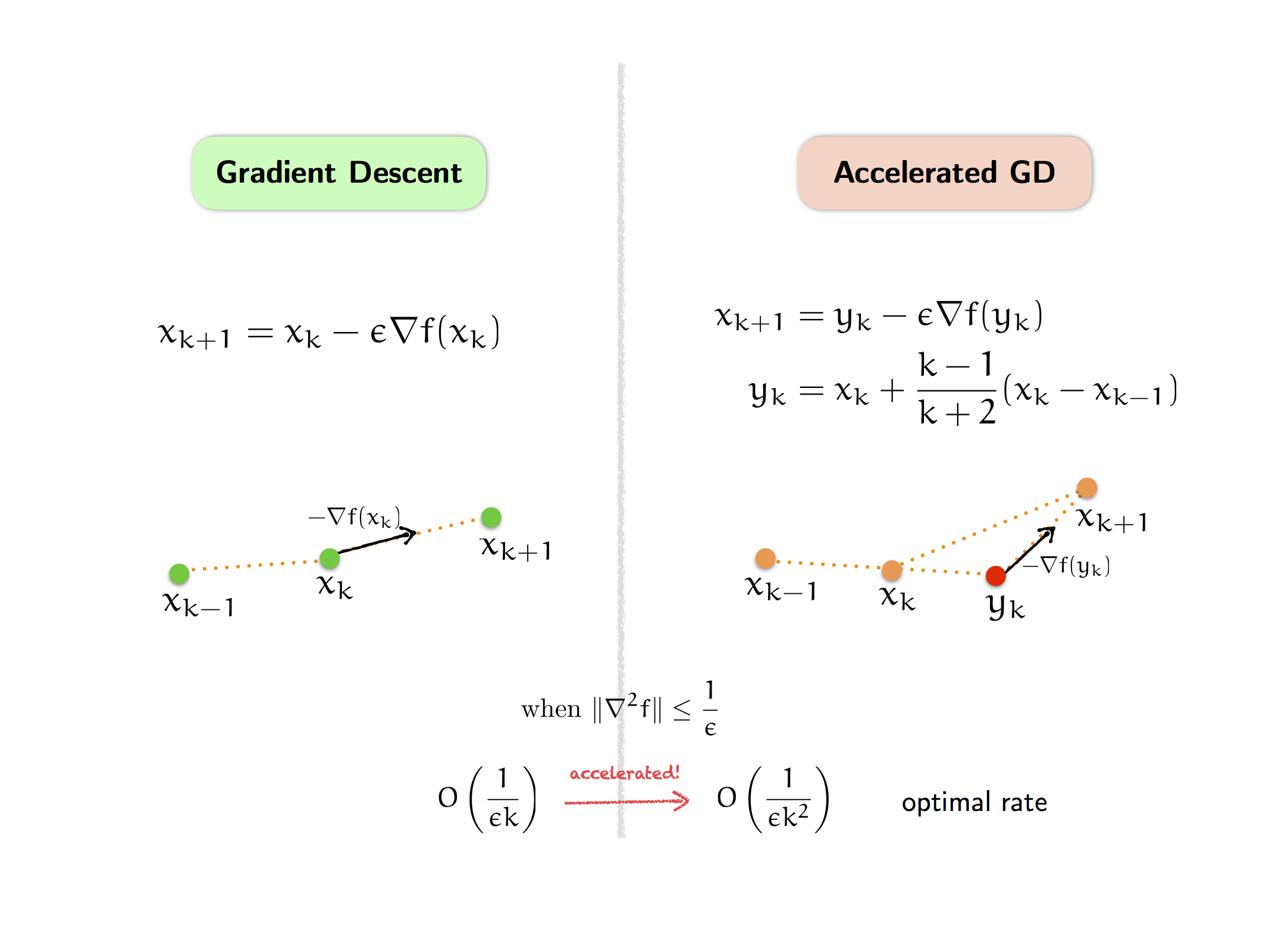
Furthermore, while gradient descent is a descent method, which means the objective function is monotonically decreasing, accelerated gradient descent is not, so the objective value oscillates. Nevertheless, accelerated gradient descent achieves a faster (and optimal) convergence rate than gradient descent under the same assumption. This is the basic view of the acceleration phenomenon, which turns out to hold much more generally in convex optimization, as we shall explore further.

Remark: As presented in Nesterov ‘04, the same acceleration phenomenon also holds when the objective function $f$ is $(1/\epsilon)$-smooth and $\sigma$-strongly convex (our discussion above is the case $\sigma = 0$). In this case, recall that gradient descent converges linearly at a rate proportional to the inverse condition number $\kappa = \epsilon \sigma$. However, gradient descent is suboptimal since the optimal rate has linear dependence on $\sqrt{\kappa}$, and it is also achieved by accelerated gradient descent, suitably modified to incorporate $\sigma > 0$. (However, in general we like to focus on the smooth case, without strong convexity, because we want to understand better the simple setting under minimum assumption, especially in continuous time.)

The mystery of acceleration

After the proposal of accelerated gradient descent in 1983 (and its popularization in Nesterov’s 2004 textbook), there have been many other accelerated methods developed for various problem settings, many of which by Nesterov himself following the technique of estimate sequence, including to the non-Euclidean setting in 2005, to higher-order algorithms in 2008, and to universal gradient methods in 2014. Estimate sequence has also been extended further to all higher-order methods by Baes in 2009.

However, many have complained that the derivation is not intuitive and looks like an “algebraic trick”. Thus, recently there have been many attempts at proposing alternate explanations or interpretations of accelerated methods, including the following selected examples.

For a quadratic objective function, as explained in this excellent post by Moritz Hardt, accelerated gradient descent is equivalent to using the Chebyshev polynomial, which provides a more efficient polynomial approximation to the inverse function, and in turn translates to a faster convergence rate for optimization.

Allen-Zhu and Orecchia emphasize the linear coupling (the “ultimate unification”) of gradient descent and mirror descent as the main force behind acceleration, as already formulated in Nesterov ‘05.

An interesting point of view is to understand accelerated gradient descent as the “optimal” first-order method. For instance, we can unfold the recursion defining accelerated gradient descent and write $x_{k+1}$ as a linear combination of the previous gradients:

$$x_{k+1} = y_0-\epsilon \sum_{i=0}^k \alpha_{k,i} \nabla f(y_i)$$

for some appropriate coefficients $(\alpha_{k,i})$, $0 \le i \le k-1$, which can be computed and turn out to look parabolic, as plotted below for $k \le 100$:

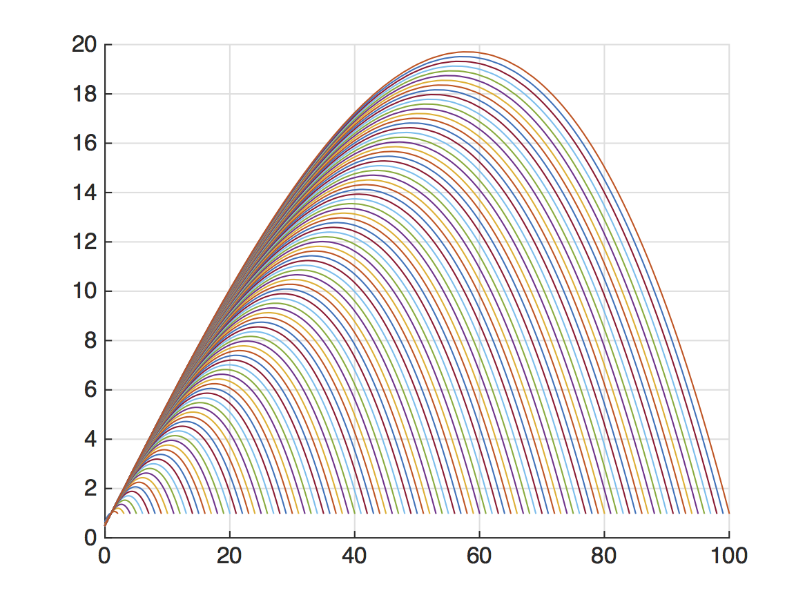
(for comparison, note that for gradient descent the coefficients are all $1$: $x_{k+1} = x_0 - \epsilon \sum_{i=0}^k \nabla f(x_i)$). Then we can find the optimal first-order method by optimizing over all possible coefficients, which can be formulated as a huge semidefinite programming that can be solved exactly, and the optimal solution actually recovers accelerated gradient descent; see this paper by Kim and Fessler and this follow-up work by Taylor et al.

There are many others, and indeed in recent years the topic of acceleration has enjoyed a resurgence of interests. Yet, despite the flurry of activities, there remains a mystery to what acceleration is really doing. Many of the proposed explanations concern specific cases (such as quadratic $f$) or assume strong assumptions (such as strong convexity). Moreover, all of the proposed theories are only for first-order methods, whereas we have seen that there are accelerated higher-order methods as in Nesterov ‘08 and Baes ‘09.

Therefore, there is still a question of what is the underlying mechanism that generates acceleration, in particular one that includes higher-order methods? In this series of posts (which is based on a joint work with Ashia Wilson and our advisor Michael Jordan) we attempt to answer this question. In particular, we provide a variational perspective—which means we interpret accelerated methods as the optimal solution to a larger optimization problem—and furthermore, we do so in continuous time via the principle of least action, which is a fundamental principle that underlies all of physics. Ultimately, our goal is to discuss the Bregman Lagrangian, which is a functional that generates all accelerated methods in continuous time.

As a closing thought, note that the acceleration phenomenon means there is something interesting going on in the world of convex optimization, in which the simple greedy action (gradient descent) is too simple, and we can do better by exploiting some non-trivial structure in the world (accelerated gradient descent); we shall see how this structure extends to a great generality in the world of convex optimization, in both continuous and discrete time.

The origin: Part 3