Hamiltonian

$\def \R {\mathbb R} \def \X {\mathcal X} \def \L {\mathcal L} \def \TqQ {\mathsf{T}_qQ} \def \H {\mathcal H} \def \E {\mathcal E} \newcommand{part}[2]{\frac{\partial #1}{\partial #2}}$ Last time, we saw how the Hamiltonian

$$\H = p \dot q - \L$$

arises as a conserved quantity when the Lagrangian $\L = \L(q, \dot q)$ has time-translation invariance (i.e., has no explicit dependence on time). Here

$$p = \frac{\partial \L}{\partial \dot q}$$

is the momentum variable conjugate to position.

For the ideal Lagrangian $\L = \frac{m}{2}\dot q^2 - V(q)$ from classical mechanics, momentum is proportional to velocity, $p = m \dot q$, and the Hamiltonian is the energy, $\H = \frac{m}{2}\dot q^2 + V(q)$, which is conserved.

More generally, if the Lagrangian $\L = \L(q, \dot q, t)$ depends on time, then the Hamiltonian $\H = \H(q,p,t)$ also depends on time, and is no longer conserved. However, we still define the momentum as $p = \frac{\partial \L}{\partial \dot q}$, which now also depends on time, and use the same formula $\H = p \dot q - \L$.

The Hamiltonian $\H$ turns out to be a very central object in physics, especially quantum mechanics, where it serves as the generator of the time evolution operator. Furthermore, it turns out we can reformulate Lagrangian mechanics from an equivalent Hamiltonian perspective in phase space $(q,p)$ that gives an equal footing to position and momentum, and has a beautiful underlying symplectic geometry with many nice properties, for example volume preservation (Liouville’s theorem).

As before, we follow Susskind’s presentation in the Classical Mechanics course, Lectures 6 and 7.

Hamiltonian dynamics

The prerequisite for translating Lagrangian dynamics into Hamiltonian is to be able to solve for $\dot q$ from the equation $p = \frac{\partial \L}{\partial \dot q}$ defining momentum, so $q$ and $p$ are the fundamental variables in the dynamics, rather than $q$ and $\dot q$. (As Susskind said, unless we can do this, the system in consideration cannot come from quantum mechanics, because the Hamiltonian is the most important thing there.)

Now we can think of the Hamiltonian

$$\H = p \dot q - \L$$

as a function of $(q,p)$. If we make a small change $(\delta q, \delta p)$ to it, then the change in $\H$ is

$$\delta \H \;=\; \dot q \: \delta p + p \: \delta \dot q - \frac{\partial \L}{\partial q} \: \delta q - \frac{\partial \L}{\partial \dot q} \: \delta \dot q \;=\; \dot q \: \delta p - \dot p \: \delta q$$

where we have used the defining relation $p = \partial \L / \partial \dot q$, and the Euler-Lagrange equation $\dot p = \partial \L / \partial q$.

But in general, we also have $\delta \H = \frac{\partial \H}{\partial p} \, \delta p + \frac{\partial \H}{\partial q} \, \delta q$. Comparing these two expansions, we must have

$$\begin{align*} \part{H}{p} &= \dot q \\ \part{H}{q} &= -\dot p \end{align*}$$

These are the Hamilton’s equations of motion, which are equivalent to the Euler-Lagrange equation. Observe how parallel $p$ and $q$ play a role above—except for the negative sign, which introduces the symplectic structure which makes the Hamiltonian formalism so nice. And notice that Hamilton’s equations are first-order in time, and there are twice as many of them as the second-order Euler-Lagrange equation.

However, also note that rather than being a gradient flow, Hamiltonian dynamics is a symplectic flow since we “rotate” the gradient vector by applying the symplectic form in phase space. That is, if we denote $z = (q,p)$ and the Hamiltonian as $\H(z)$, then we can write Hamilton’s equations as vector field

$$\dot z = J \, \nabla \H(z)$$

where we apply the symplectic matrix

$$J = \begin{pmatrix} 0 & 1 \\ -1 & 0 \end{pmatrix}$$

to the usual gradient vector $\nabla \H(z) = (\part{\H}{q}, \part{\H}{p})^\top$, so we indeed recover Hamilton’s equations

$$\begin{pmatrix} \dot q \\ \dot p \end{pmatrix} = \begin{pmatrix} 0 & 1 \\ -1 & 0 \end{pmatrix} \begin{pmatrix} \part{\H}{q} \\ \part{\H}{p} \end{pmatrix} = \begin{pmatrix} \part{\H}{p} \\ -\part{\H}{q} \end{pmatrix}$$

And notice, the symplectic matrix $J$ is the same as rotation by $270^\circ$ in the phase space. Thus, instead of following the gradient $\nabla \H(z)$ (like gradient flow), the Hamiltonian dynamics goes perpendicular to it. Recall, the gradient of a function is the direction of largest increase, which is orthogonal to the level set (contour surface). This means the Hamiltonian dynamics always travels parallel to the level set of the Hamiltonian $\H$. Furthermore, since this is true for each time, the dynamics always stays on the same level set of $\H$, which means the Hamiltonian is conserved!

Note that the last sentence above only holds when the Hamiltonian is time-independent, since otherwise the level set also changes with time. More generally, when the Hamiltonian $\H = \H(q,p,t)$ depends on time, its total time derivative is equal to the partial derivative with respect to time:

$$\frac{d\H}{dt} = \part{\H}{q} \dot q + \part{\H}{p} \dot p + \part{\H}{t} = \part{\H}{t}$$

where the first two terms above cancel because of Hamilton’s equations.

Example: Harmonic oscillator

Consider the Lagrangian for the harmonic oscillator

$$\L= \frac{1}{2\omega} \dot q^2 - \frac{\omega}{2} q^2$$

where $\omega = \sqrt{k/m}$ is a convenient parameterization that is the fundamental frequency, where $m$ is mass and $k$ is spring constant. The momentum variable is $p = \frac{\partial \L}{\partial \dot q} = \frac{1}{\omega} \dot q$, so we can solve for $\dot q = \omega p$.

Then we can write the Hamiltonian as a function of $p$ and $q$:

$$\H(q,p) = p \dot q - \L = \omega p^2 - \left(\frac{1}{2\omega} (\omega p)^2 - \frac{\omega}{2} q^2 \right) = \frac{\omega}{2} (p^2+q^2)$$

So the Hamiltonian, or the energy, is proportional to the squared radius $p^2 + q^2$ in phase space. Conservation of energy means the trajectory in phase space is constrained to lie on a circle, and indeed by Hamilton’s equations

$$\begin{align*} \dot q &= \omega p \\ \dot p &= -\omega q \end{align*}$$

which means every point has a circular orbit, so the whole phase space rotates with the same angular frequency $\omega$ like a rigid pinwheel (figure below from Perlick’s lecture notes).

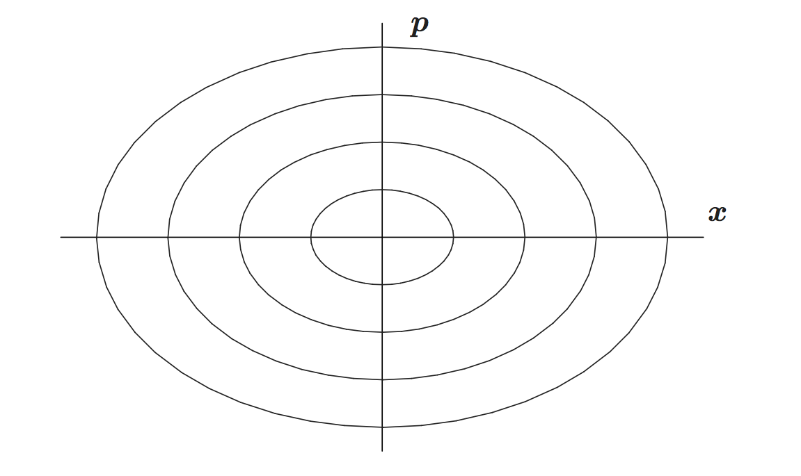
Notice that if we differentiate the first equation above and subsitute the second equation, we get

$$\ddot q = \omega \dot p = -\omega^2 q$$

which is the familiar Euler-Lagrange equation for the harmonic oscillator with frequency $\omega = \sqrt{k/m}$.

Liouville's theorem

As Susskind emphasized, the “$-1^{\text{st}}$ law” in physics is the law of reversibility, whose ultimate meaning is that we never lose information. Concretely, this means if two states are distinguishable at some time, then they must be distinguishable at all time.

Therefore, dynamics are just reshuffling of states. When the state space is finite, the dynamics are permutations (see also Susskind’s Lecture 1). On the other hand, when the state space is continuous (like our phase space), the allowable dynamics are measure-preserving transformations.

We will see that the flow generated by Hamilton’s equations of motion is always a measure-preserving transformation. This means if we take a little region in phase space and track its evolution under the Hamiltonian flow, we will find that the volume of the region is always the same at each time.

This is the preservation of volume in phase space, known as Liouville’s theorem. Here “volume” means the Lebesgue measure in phase space, and the theorem states that the Hamiltonian flow pushes the Lebesgue measure forward to itself (hence “measure-preserving”). This is also essentially the same as Heisenberg’s uncertainty principle in quantum mechanics.

The above is a “Lagrangian” description of the dynamics, where we follow the trajectory of a particle. There is also an equivalent “Eulerian” description, where we fix a point $(q,p)$ in space and study the velocity $v(q,p,t)$ of the particle going through that point at time $t$ (see, for example, Villani’s $\S 3.2.2$).

The Eulerian description of a measure-preserving transformation is that the generating vector field $v = (v_q, v_p)^\top$ has zero divergence:

$$\nabla \cdot v := \begin{pmatrix} \part{\,}{q} & \part{\,}{p} \end{pmatrix} \begin{pmatrix} v_q \\ v_p \end{pmatrix} = \part{v_q}{q} + \part{v_p}{p} = 0$$

which means at each point $(q,p)$ the amount that flows in is the same as what flows out. This means there are no sources or sinks, the entire phase space behaves like an incompressible fluid, as if made of little billiard balls that are being pushed around under the dynamics.

For the Hamiltonian flow above, $v_q = \part{\H}{p}$ and $v_p = -\part{\H}{q}$, so we see it indeed has zero divergence:

$$\nabla \cdot v = \part{\,}{q} \part{\H}{p} + \part{\,}{p} \left(-\part{\H}{q}\right) = 0$$

since the partial derivatives commute. This means Hamiltonian flow preserves volume in phase space. Notice, this still holds even when the Hamiltonian is time-dependent, for example when there is friction (dissipation), as we illustrate below.

The incompressibility of the Hamiltonian flow is because the symplectic form is antisymmetric, so it is zero on the diagonal. Concretely, since the Hamiltonian vector field is $v = J \nabla \H$ and the symplectic matrix $J$ is skew-symmetric, it has zero divergence:

$$\nabla \cdot v = \nabla \cdot J \, \nabla \H = \begin{pmatrix} \part{\,}{q} & \part{\,}{p} \end{pmatrix} \begin{pmatrix} 0 & 1 \\ -1 & 0 \end{pmatrix} \begin{pmatrix} \part{\,}{q} \\ \part{\,}{p} \end{pmatrix} \H = 0$$

The bottom line, as Susskind said, is that the flow associated to the law of physics should not have a divergence or convergence; that is the ultimate meaning of reversibility.

(Susskind also showed that in one dimension, the only incompressible flow is the uniform motion with constant velocity, which is like the flow of time(?).)

Damped Hamiltonian

Consider now the damped Lagrangian $\L = \L(q, \dot q, t)$

$$\L = e^{\gamma_t} \left(\frac{m}{2} \dot q^2 - V(q)\right)$$

where $\gamma \colon \R \to \R$ is an arbitrary damping function and $V \colon Q \to \R$ is the potential function. This generates an equation of motion with friction

$$m \ddot q + m \dot \gamma_t \dot q + \nabla V(q) = 0$$

for which the mechanical energy $\E = \frac{m}{2} \dot q^2 + V(q)$ is dissipated, since indeed $\dot \E = -m \dot \gamma_t \dot q^2 \le 0$. However, the Hamiltonian is not the mechanical energy, but a rescaled (damped) version of it.

First, the momentum variable is

$$p = \part{\L}{\dot q} = m e^{\gamma_t} \dot q$$

which now also depends on time, and which we can solve for $\dot q$ as

$$\dot q = \frac{1}{me^{\gamma_t}} p$$

Then the (damped) Hamiltonian $\H = \H(q,p,t)$ is

$$\H = p \dot q - \L = \frac{1}{me^{\gamma_t}} p^2 - e^{\gamma_t}\left( \frac{m}{2} \left(\frac{1}{me^{\gamma_t}} p \right)^2 - V(q) \right) = \frac{1}{2me^{\gamma_t}} p^2 + e^{\gamma_t} V(q)$$

which we can also express in terms of $q$ and $\dot q = \frac{1}{m e^{\gamma_t}} p$ as

$$\H = e^{\gamma_t} \left( \frac{m}{2} \dot q^2 + V(q) \right)$$

Thus, the Hamiltonian is the sum of the (damped) kinetic and potential energy, whereas the Lagrangian is the difference, just like in the ideal case.

However, observe that the Hamiltonian is not preserved:

$$\dot \H = \dot \gamma_t \H + e^{\gamma_t} \left( m \dot q \ddot q + \nabla V(q) \dot q \right) = \dot \gamma_t \H - m \dot \gamma_t e^{\gamma_t} \dot q^2 = - \dot \gamma_t \L \neq 0$$

but it is hard to say how the Hamiltonian behaves in general, though it seems to be decreasing(?).

The Hamiltonian equations of motion are

$$\begin{align*} \dot q &= \part{H}{p} = \frac{1}{me^{\gamma_t}} p \\ \dot p &= -\part{H}{q} = -e^{\gamma_t} \nabla V(q) \end{align*}$$

which still have zero divergence, since $\part{\,}{q} (\frac{1}{me^{\gamma_t}} p) + \part{\,}{p} (-e^{\gamma_t} \nabla V(q)) = 0$.

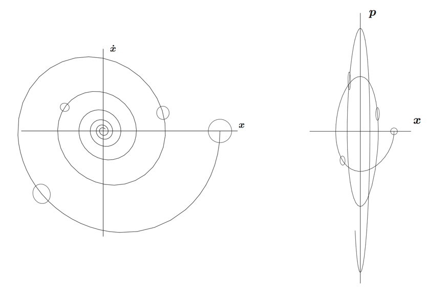
This means we have preservation of volume in phase space. This is reflected in the fact that the momentum diverges $p \to \infty$ as position converges $q \to q^\ast$, since the area has to be conserved (whereas in the $(q, \dot q)$ space the dissipative dynamics shrinks area since eventually $(q,\dot q) \to (q^\ast, 0)$).

Example: Damped harmonic oscillator

Finally, consider the damped harmonic oscillator with friction

$$m \ddot q + c \dot q + k q = 0$$

which comes from linear damping $\gamma_t = \frac{ct}{m}$ and quadratic potential $V(q) = \frac{k}{2} q^2$, so the Lagrangian is

$$\L = e^{\frac{ct}{m}} \left(\frac{m}{2}\dot q^2 - \frac{k}{2} q^2\right)$$

and the Hamiltonian is

$$\H = \frac{e^{-\frac{ct}{m}}}{2m} p^2 + \frac{e^{ct/m} k}{2} q^2$$

where the momentum is $p = me^{\frac{ct}{m}} \dot q$. The Hamiltonian equations of motion are

$$\begin{align*} \dot q &= \frac{e^{-\frac{ct}{m}}}{m} p \\ \dot p &= -e^{\frac{ct}{m}} k q \end{align*}$$

In the “underdamped” case when $\omega^2 := \frac{k}{m} - \frac{c^2}{4m^2} \ge 0$, we can solve the equations above explicitly (see for example Perlick’s Lecture 3):

$$\begin{pmatrix} q(t) \\ p(t) \end{pmatrix} = M(t) \begin{pmatrix} q(0) \\ p(0) \end{pmatrix}$$

where $M(t)$ is the time-dependent transformation matrix

$$M(t) = \begin{pmatrix} e^{-\frac{ct}{2m}}\left(\cos (\omega t) + \frac{c}{2m\omega} \sin(\omega t)\right) & e^{-\frac{ct}{2m}}\frac{1}{m\omega} \sin(\omega t) \\ -e^{\frac{ct}{2m}}\left(m\omega+\frac{c^2}{4m\omega}\right)\sin(\omega t) & e^{\frac{ct}{2m}}\left(\cos (\omega t) - \frac{c}{2m\omega} \sin(\omega t)\right) \end{pmatrix}$$

which has unit determinant, $\det(M(t)) = 1$, so it conserves the phase space volume. Thus, while the velocity $\dot q \to 0$ stabilizes, the momentum $p \to \infty$ explodes, as illustrated below (figures from Perlick).